---
title: "ACF y PACF en ARMA(p,q)"
author: "Brayan Cubides"
toc: true
toc-location: right
toc-depth: 2
#number-sections: true
code-tools: true
lightbox: true
self-contained: false
---
## ACF de modelos AR
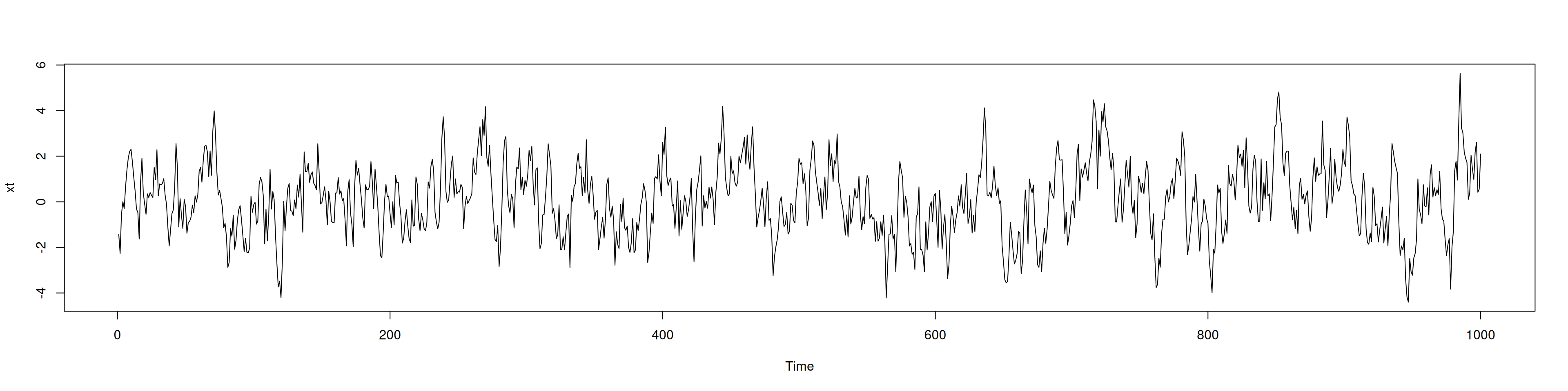
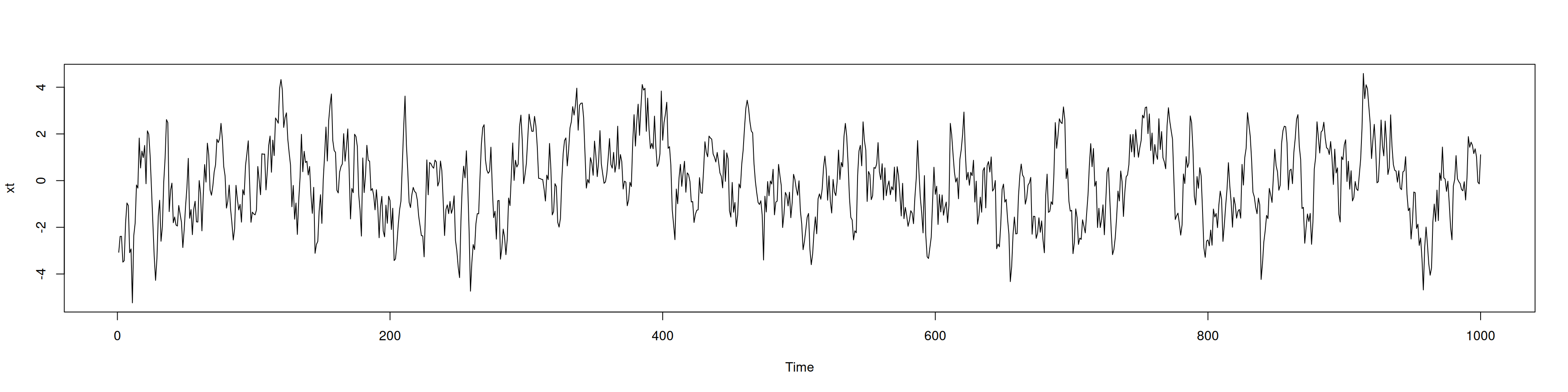
### AR(1)
```{r, fig.width=20, fig.height=5, out.width="100%"}
rm(list=ls(all=TRUE))
set.seed(123)
# Simulación AR(1)
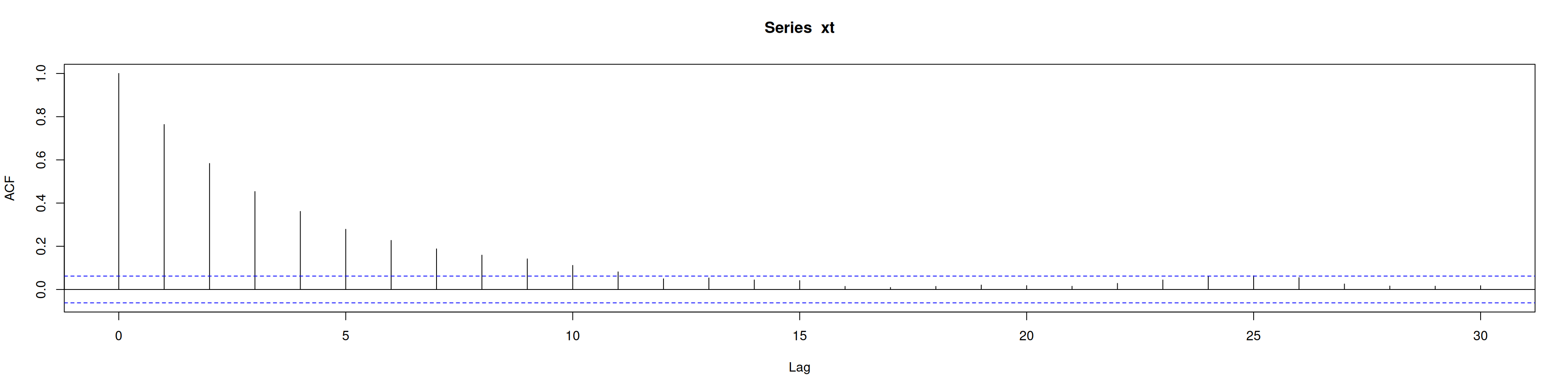
xt <- arima.sim(list(ar = c(0.79)), n = 1000)
ts.plot(xt)
acf(xt) # Decae de forma exponencial
```
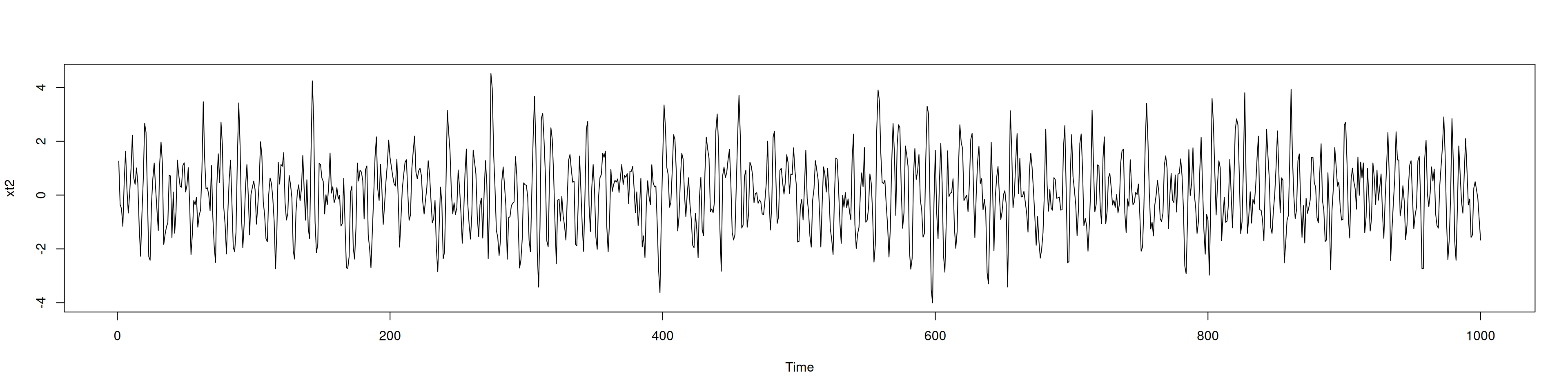
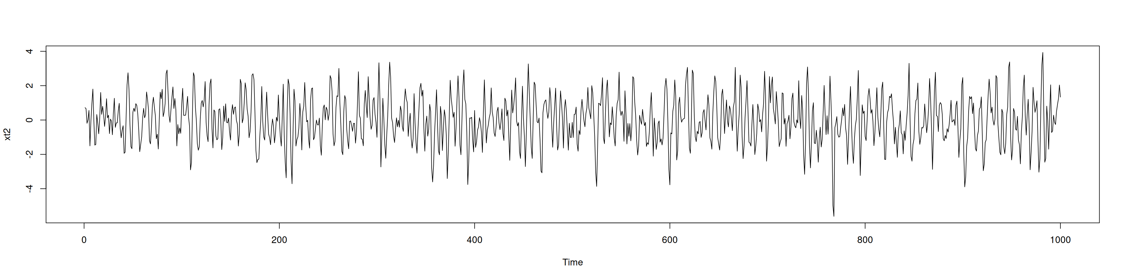
### AR(2)
```{r, fig.width=20, fig.height=5, out.width="100%"}
# Simulación AR(2) con coeficientes 0.8 y -0.55
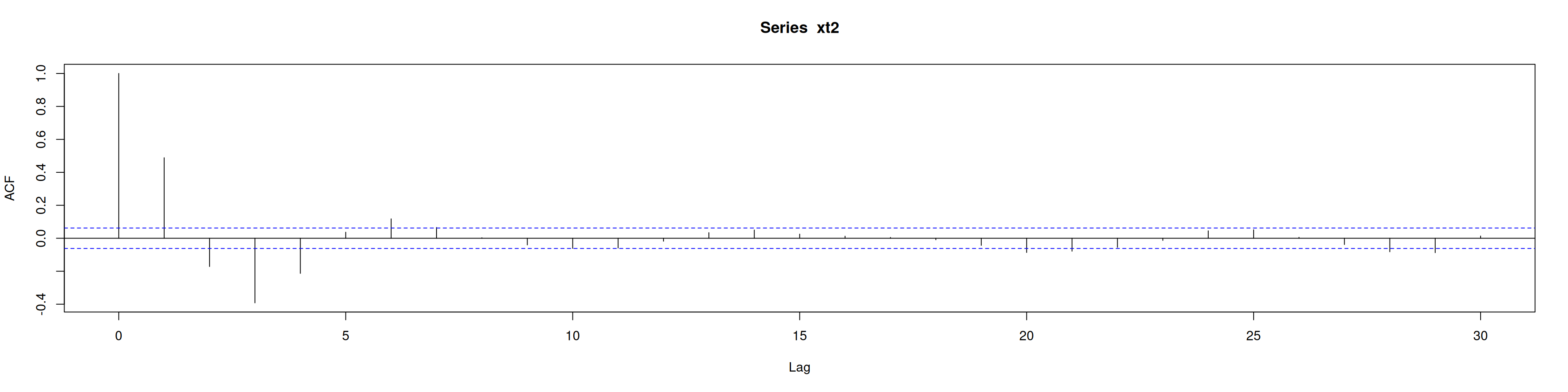
xt2 <- arima.sim(list(order = c(2,0,0), ar = c(0.8, -0.55)), n = 1000)
ts.plot(xt2)
acf(xt2)
```
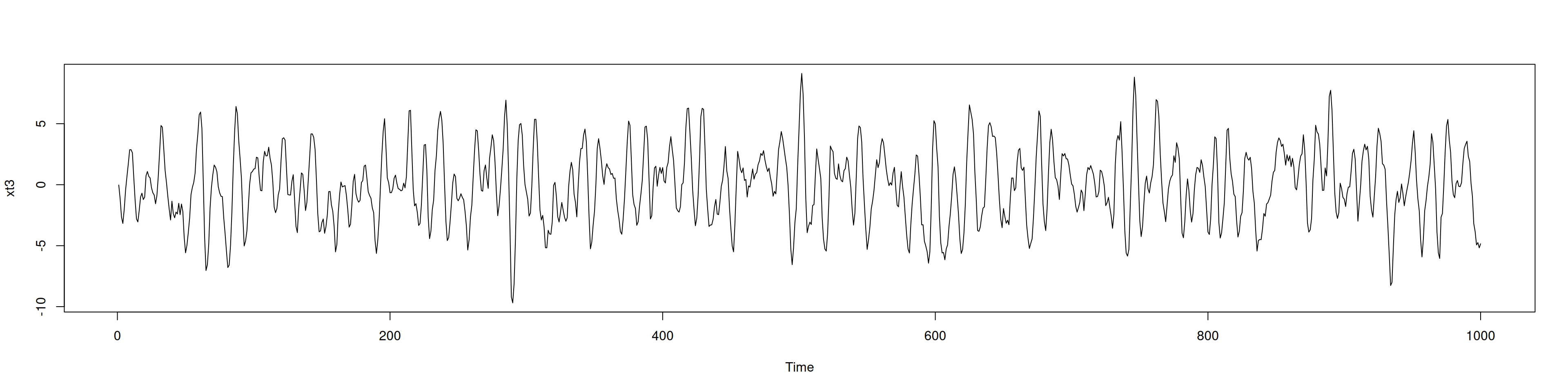
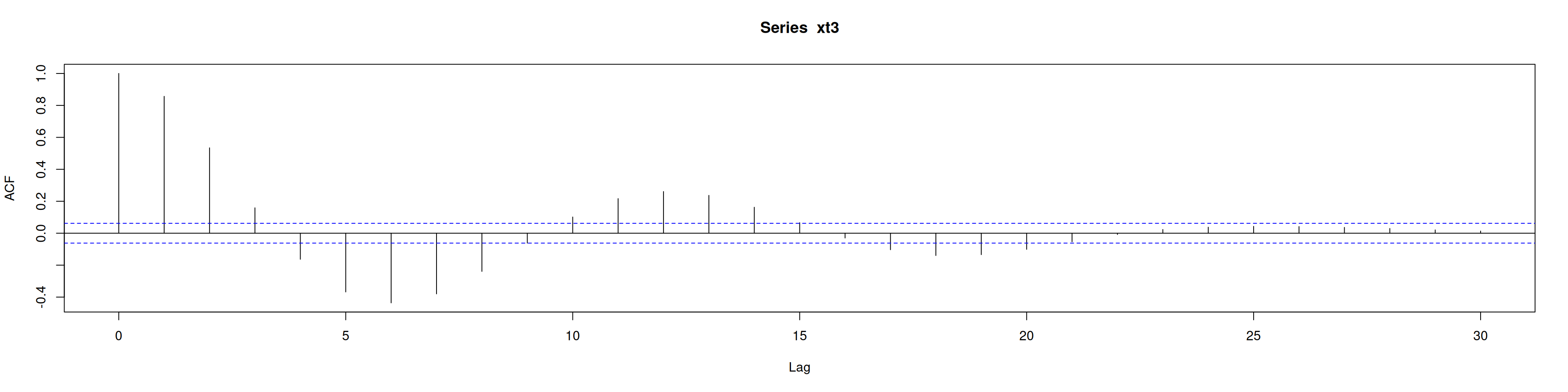
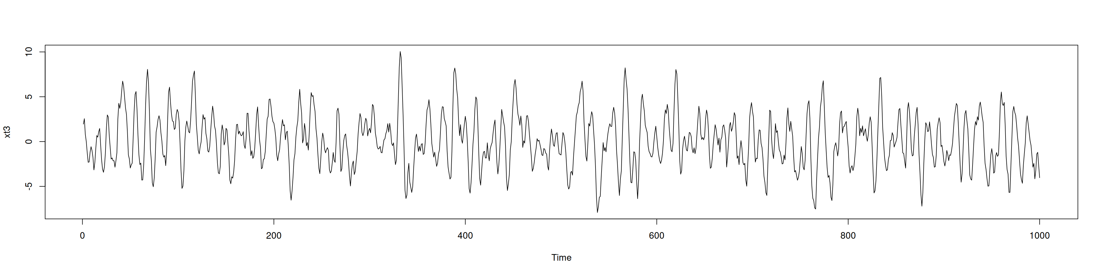
### AR(2) no estacionario (Diapositiva 52)
```{r, fig.width=20, fig.height=5, out.width="100%"}
# Simulación AR(2) con coeficientes 1.5 y -0.75
xt3 <- arima.sim(list(order = c(2,0,0), ar = c(1.5, -0.75)), n = 1000)
ts.plot(xt3)
acf(xt3) # Decae de forma sinusoidal
```
## ACF de modelos MA
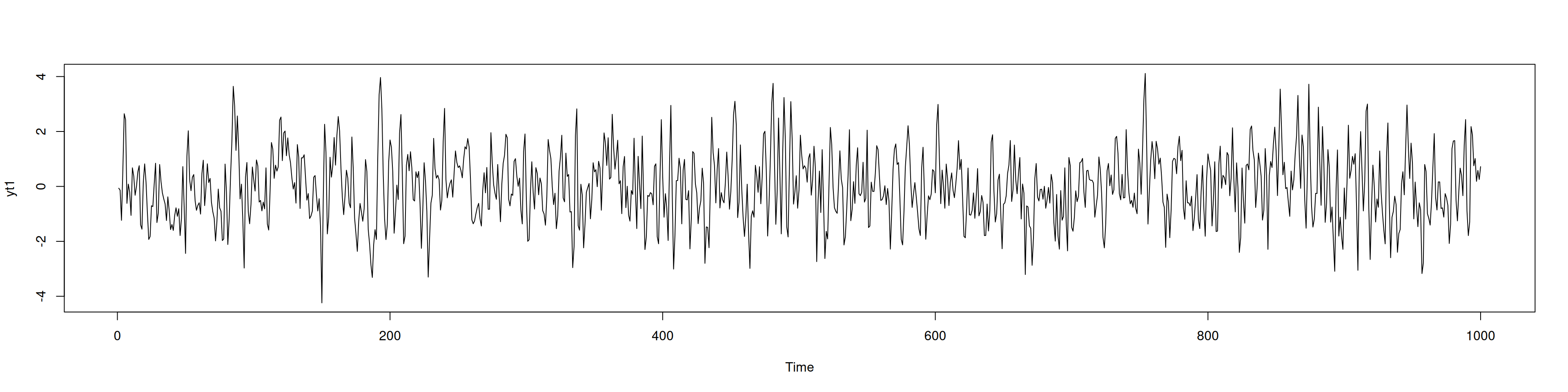
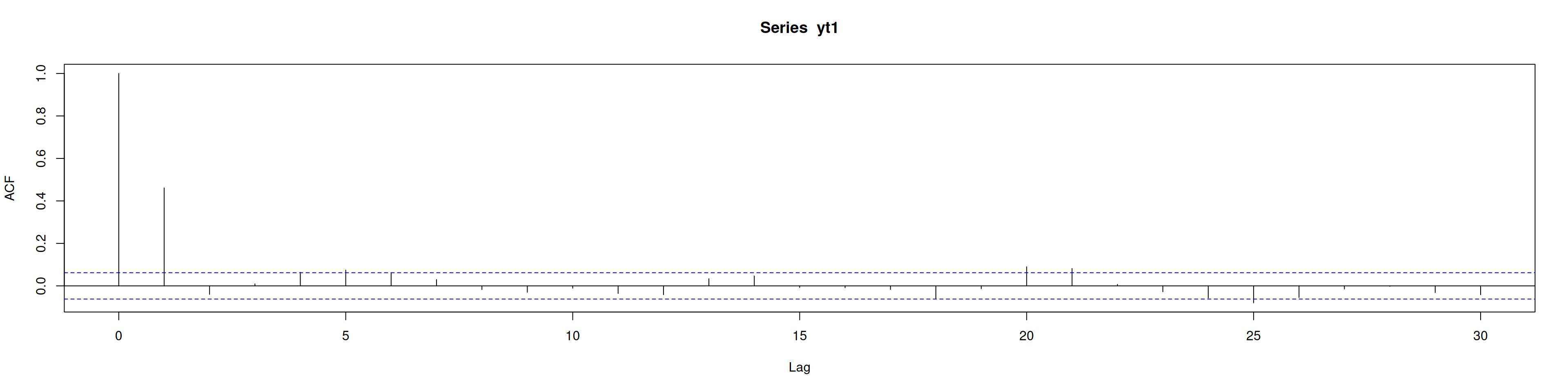
### MA(1) positiva
```{r, fig.width=20, fig.height=5, out.width="100%"}
yt1 <- arima.sim(list(ma = c(0.8)), n = 1000)
ts.plot(yt1)
acf(yt1)
```
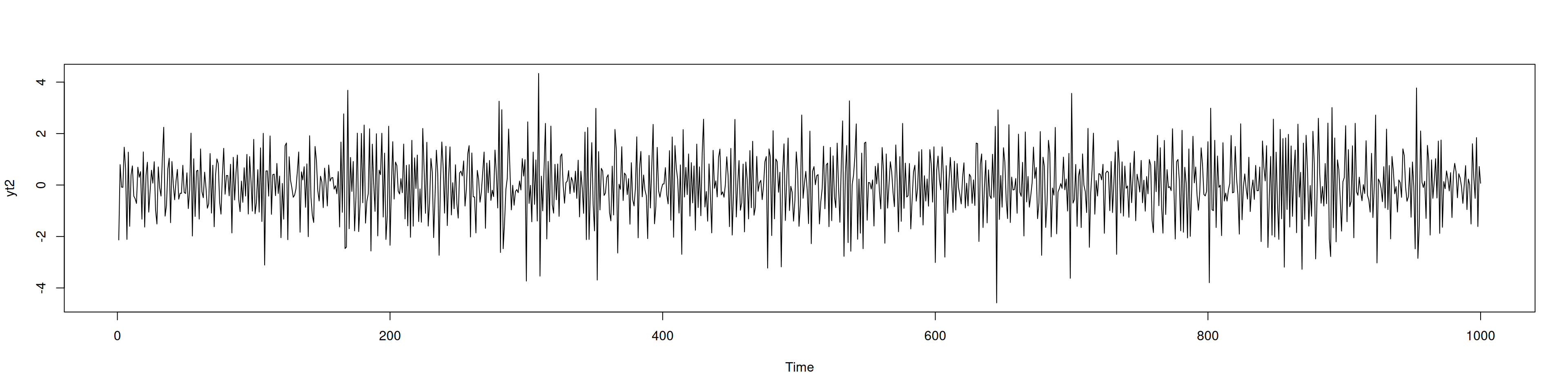
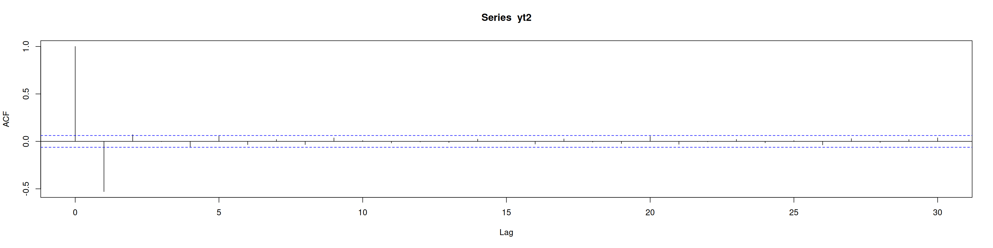
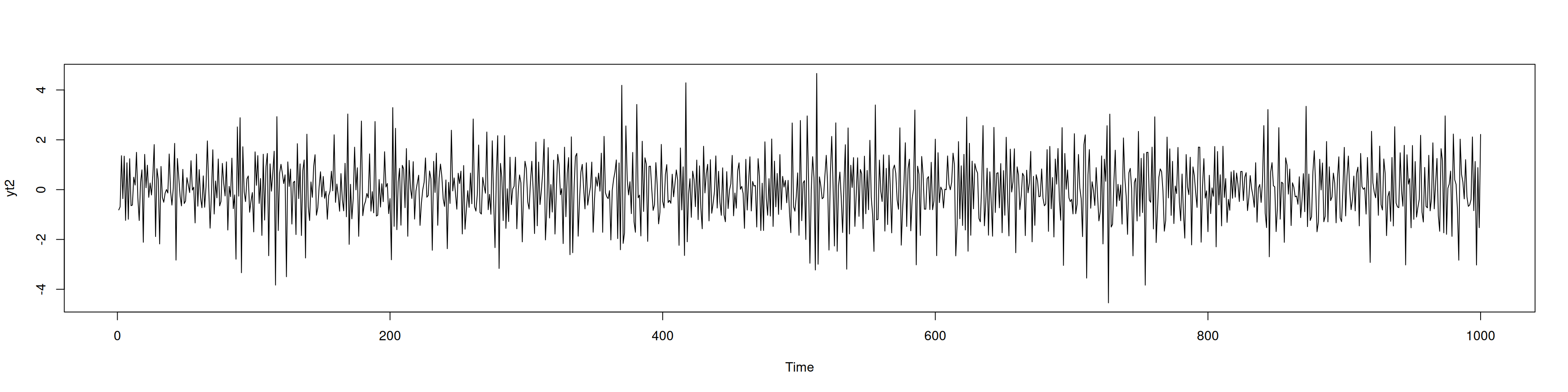
### MA(1) negativa
```{r, fig.width=20, fig.height=5, out.width="100%"}
yt2 <- arima.sim(list(ma = c(-0.8)), n = 1000)
ts.plot(yt2)
acf(yt2)
```
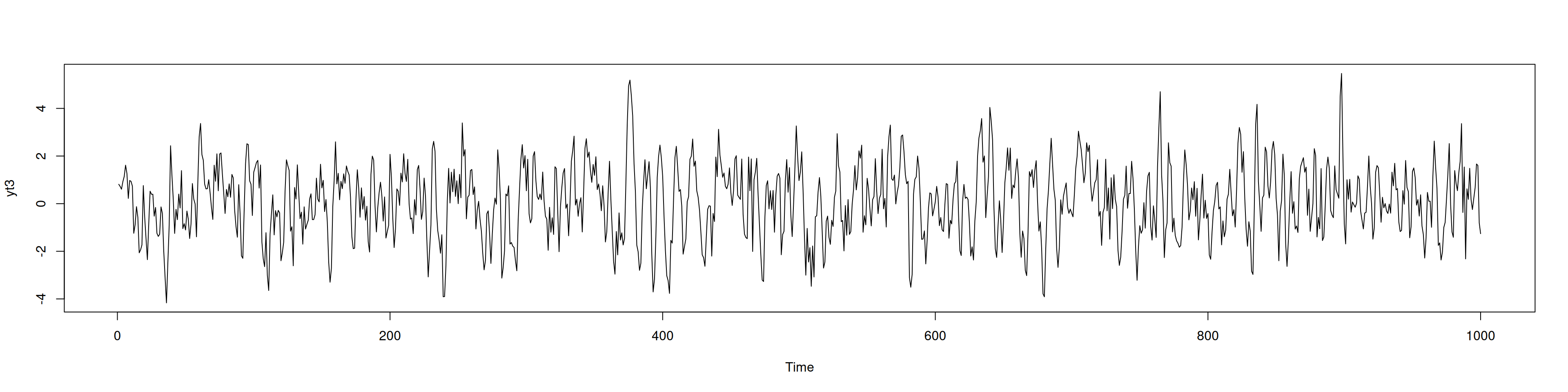
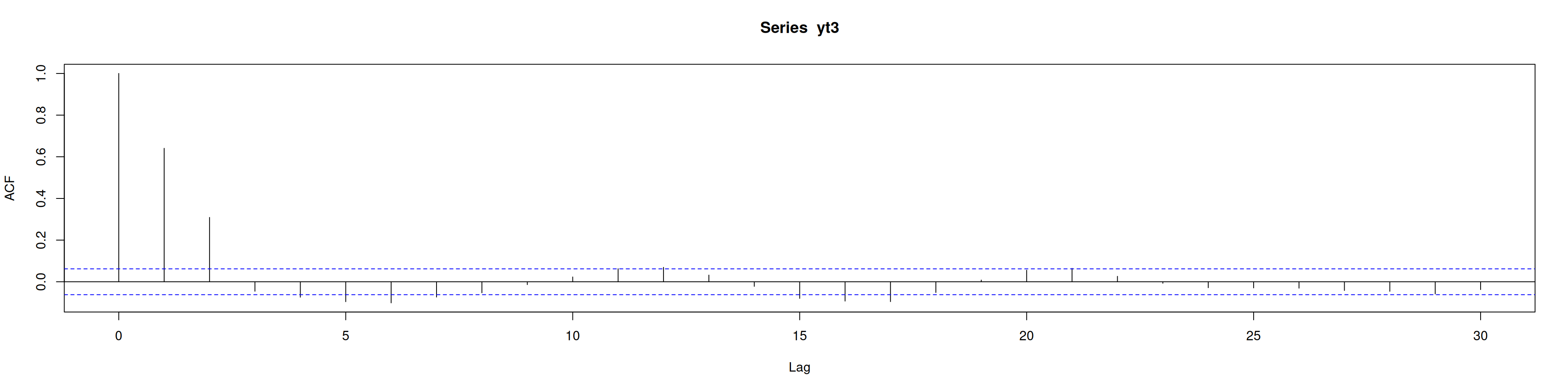
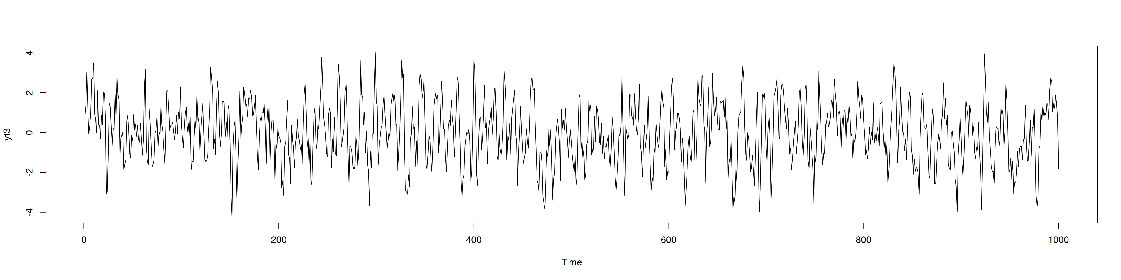
### MA(2)
```{r, fig.width=20, fig.height=5, out.width="100%"}
yt3 <- arima.sim(list(ma = c(0.9, 0.8)), n = 1000)
ts.plot(yt3)
acf(yt3)
```
## PACF de modelos AR
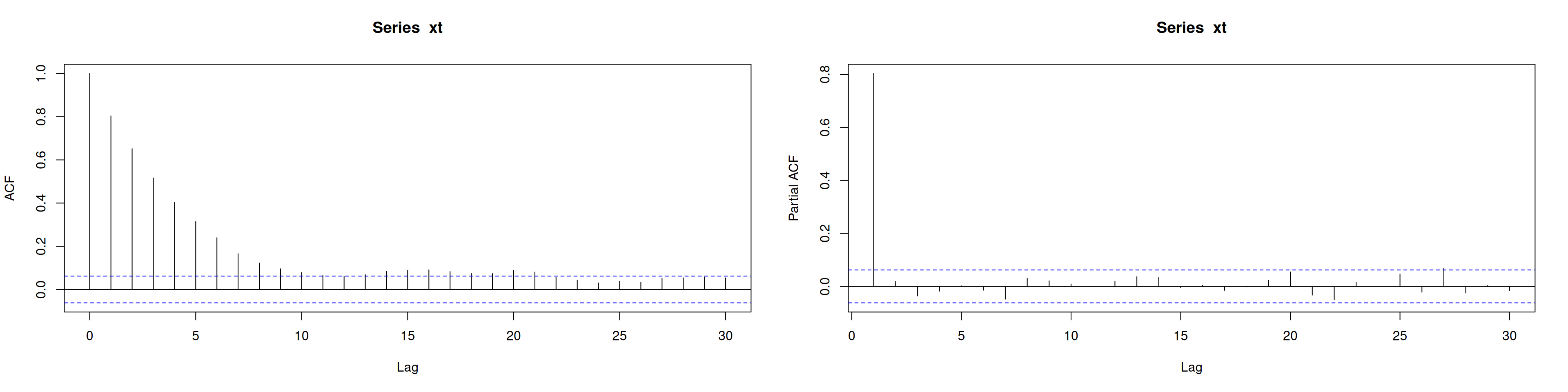
### AR(1)
```{r, fig.width=20, fig.height=5, out.width="100%"}
xt <- arima.sim(list(ar = c(0.79)), n = 1000)
ts.plot(xt)
par(mfrow = c(1,2))
acf(xt)
pacf(xt)
```
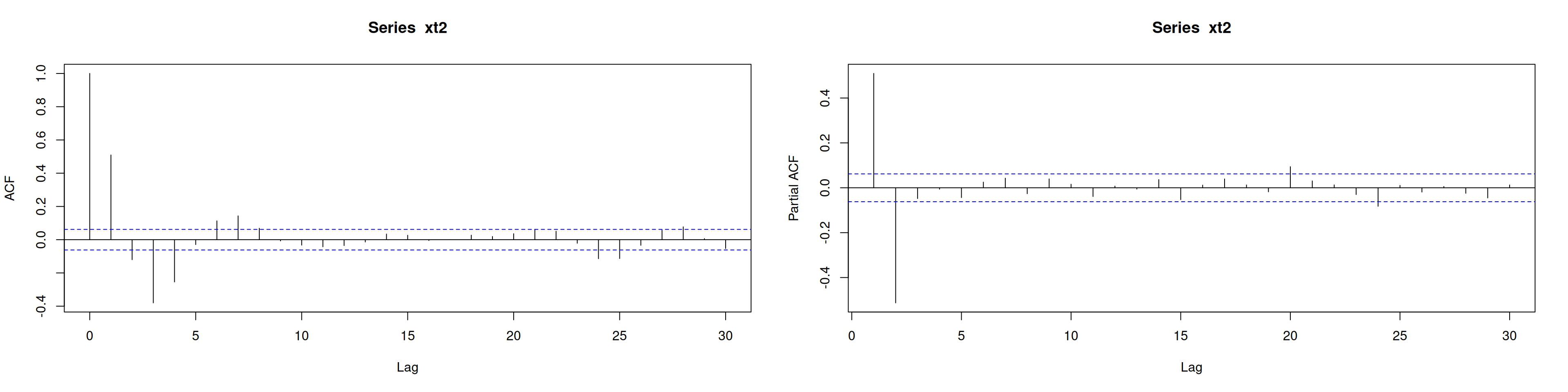
### AR(2)
```{r, fig.width=20, fig.height=5, out.width="100%"}
xt2 <- arima.sim(list(order = c(2,0,0), ar = c(0.8, -0.55)), n = 1000)
ts.plot(xt2)
par(mfrow = c(1,2))
acf(xt2)
pacf(xt2)
```
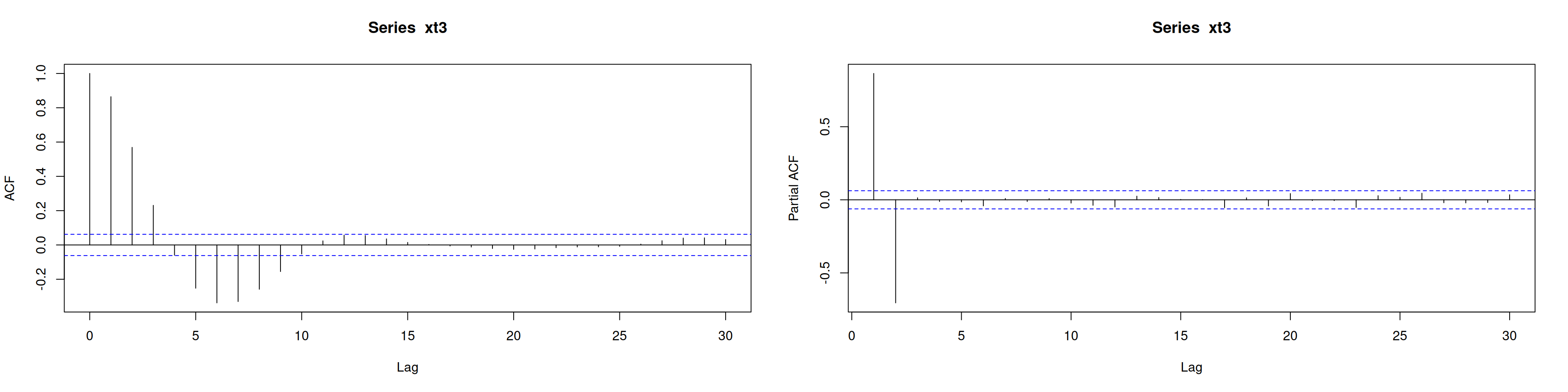
### AR(2) no estacionario
```{r, fig.width=20, fig.height=5, out.width="100%"}
xt3 <- arima.sim(list(order = c(2,0,0), ar = c(1.5, -0.75)), n = 1000)
ts.plot(xt3)
par(mfrow = c(1,2))
acf(xt3)
pacf(xt3)
```
## PACF de modelos MA
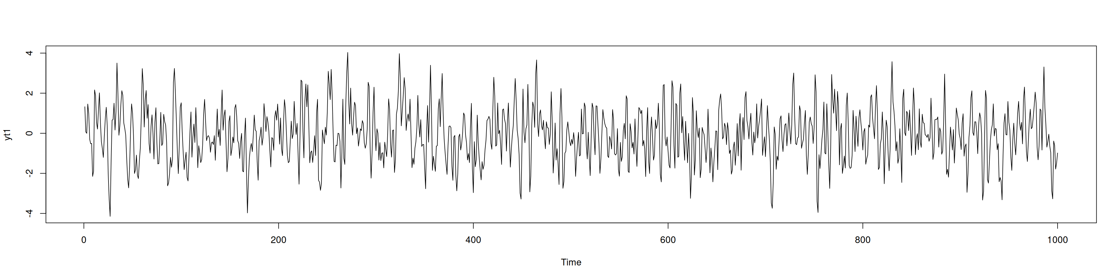
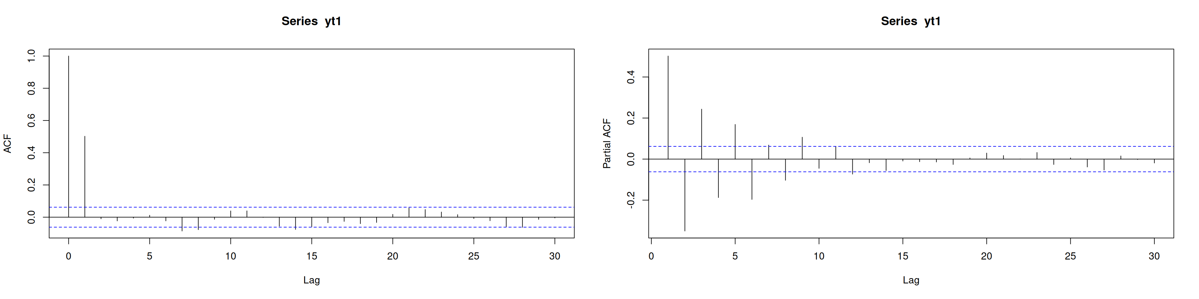
### MA(1) positiva
```{r, fig.width=20, fig.height=5, out.width="100%"}
yt1 <- arima.sim(list(ma = c(0.88)), n = 1000)
ts.plot(yt1)
par(mfrow = c(1,2))
acf(yt1)
pacf(yt1)
```
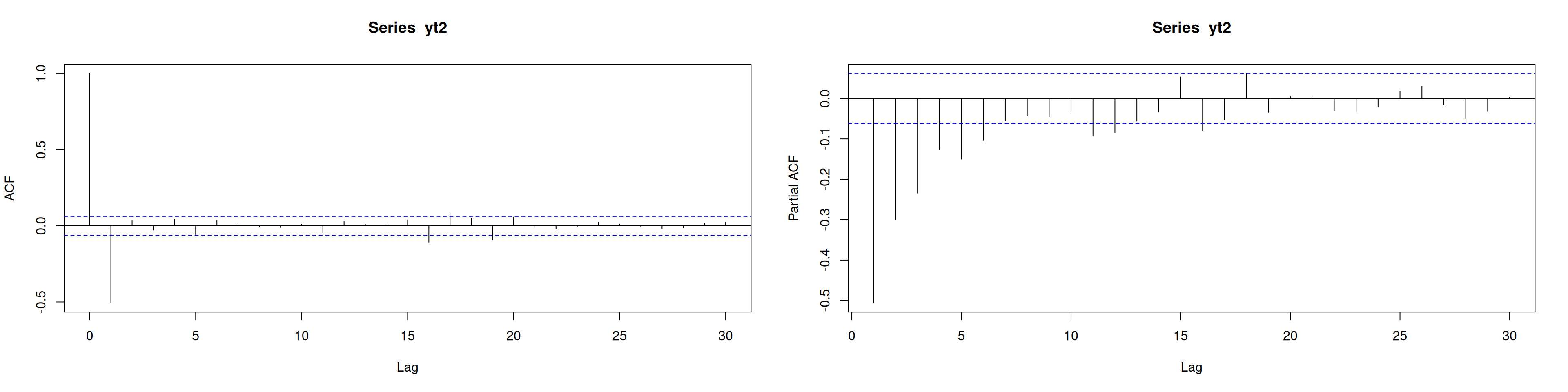
### MA(1) negativa
```{r, fig.width=20, fig.height=5, out.width="100%"}
yt2 <- arima.sim(list(ma = c(-0.8)), n = 1000)
ts.plot(yt2)
par(mfrow = c(1,2))
acf(yt2)
pacf(yt2)
```
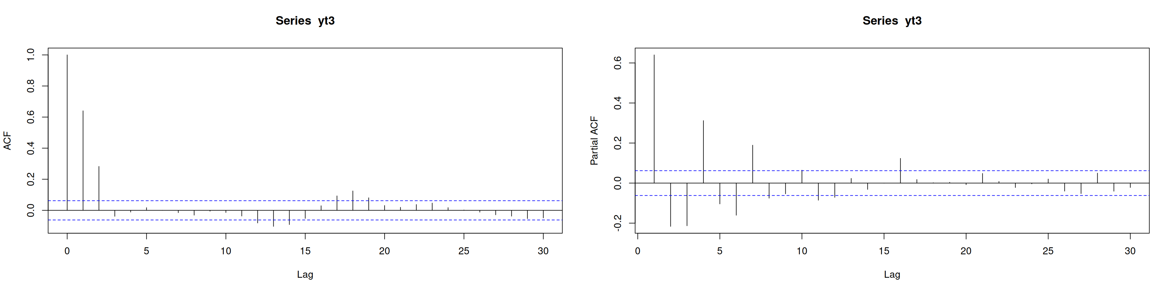
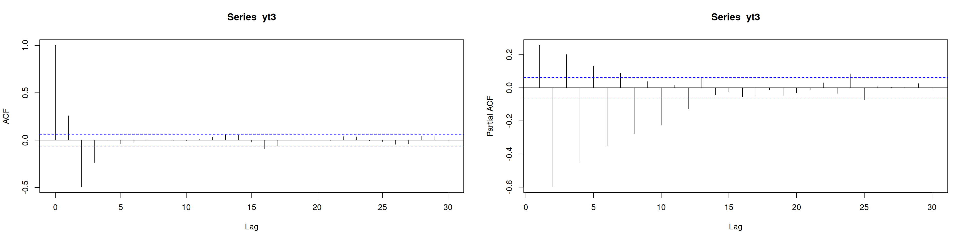
### MA(2)
```{r, fig.width=20, fig.height=5, out.width="100%"}
yt3 <- arima.sim(list(ma = c(0.9, 0.8)), n = 1000)
ts.plot(yt3)
par(mfrow = c(1,2))
acf(yt3)
pacf(yt3)
```
## Ejemplos adicionales con desviación estándar distinta
```{r, fig.width=20, fig.height=5, out.width="100%"}
# AR(2) con sd = 1.5
xt2 <- arima.sim(list(order = c(2,0,0), ar = c(0.2, 0.55)), sd = 1.5, n = 1000)

# MA(3) con sd = 3
yt3 <- arima.sim(list(ma = c(0.9, -0.8, -0.8)), sd = 3, n = 1000)
par(mfrow = c(1,2))
acf(yt3)
pacf(yt3)
```