11  Ajuste SARIMA (Completo)

12 Ejercicio de ajuste modelo SAIMA

Ajuste de la serie de pasajeros basada en Time Series Analysis - With Applications in R, 2nd Ed.

---

12.1 Librerías necesarias

library(urca)
library(forecast)
library(tseries)
library(lmtest)
library(uroot)
library(fUnitRoots)
library(aTSA)

---

12.2 Parte 1: Raíz Unitaria

Se simula un ARIMA(1,1,1) y se prueban raíces unitarias.
La prueba ADF considera: \[ \Delta X_t = \rho\,X_{t-1} + \sum_{j=1}^p\beta_j\,\Delta X_{t-j} + e_t. \]

# Raiz Unitaria
Tlength = 200
arimaej_raiz_unit = arima.sim(list(order = c(1,1,1), ar = 0.7, ma = 0.6),
                              n = Tlength)
layout(matrix(c(1,1,2, 1,1,3), nc = 2))
par(mar=c(3,3,2,1), mgp=c(1.6,.6,0))
plot(arimaej_raiz_unit)
acf(arimaej_raiz_unit)
pacf(arimaej_raiz_unit)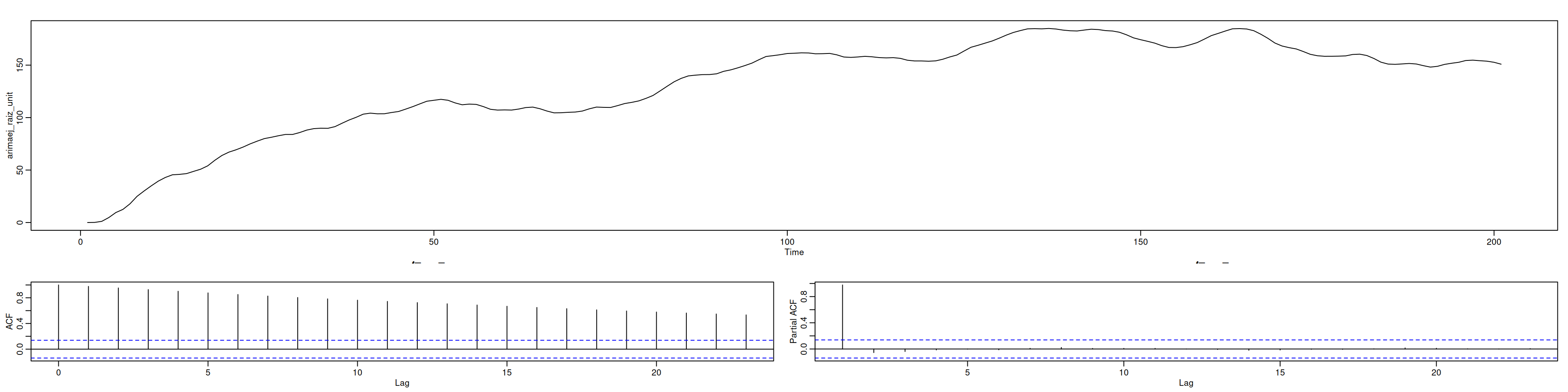

# Ho: Raiz unitaria (no estacionaria) vs Ha: Estacionariedad
tseries::adf.test(arimaej_raiz_unit)       # p.valor>0.05 ⇒ no rechaza Ho

    Augmented Dickey-Fuller Test

data:  arimaej_raiz_unit
Dickey-Fuller = -2.0267, Lag order = 5, p-value = 0.5649
alternative hypothesis: stationary

# Prueba KPSS (Ho: estacionariedad vs Ha: raiz unitaria)
tseries::kpss.test(arimaej_raiz_unit)      # p.valor<0.05 ⇒ rechaza estacionariedad

Warning in tseries::kpss.test(arimaej_raiz_unit): p-value smaller than printed
p-value

    KPSS Test for Level Stationarity

data:  arimaej_raiz_unit
KPSS Level = 3.2643, Truncation lag parameter = 4, p-value = 0.01

# Prueba Phillips-Perron (Ho: raiz unitaria vs Ha: estacionariedad)
tseries::pp.test(arimaej_raiz_unit)        # p.valor>0.05 ⇒ no rechaza Ho

    Phillips-Perron Unit Root Test

data:  arimaej_raiz_unit
Dickey-Fuller Z(alpha) = -3.5774, Truncation lag parameter = 4, p-value
= 0.9076
alternative hypothesis: stationary

Interpretación:
Las pruebas ADF y PP no rechazan raíz unitaria, mientras KPSS rechaza estacionariedad ⇒ la serie simulada no es estacionaria.

---

12.3 Parte 2: Transformación y raíces unitarias en AirPassengers

12.3.1 2.1 Estabilizar varianza

Box–Cox indica \(\lambda\approx0\) ⇒ aplicar \(\log\):

data("AirPassengers")
par(mfrow=c(1,1))
plot(AirPassengers)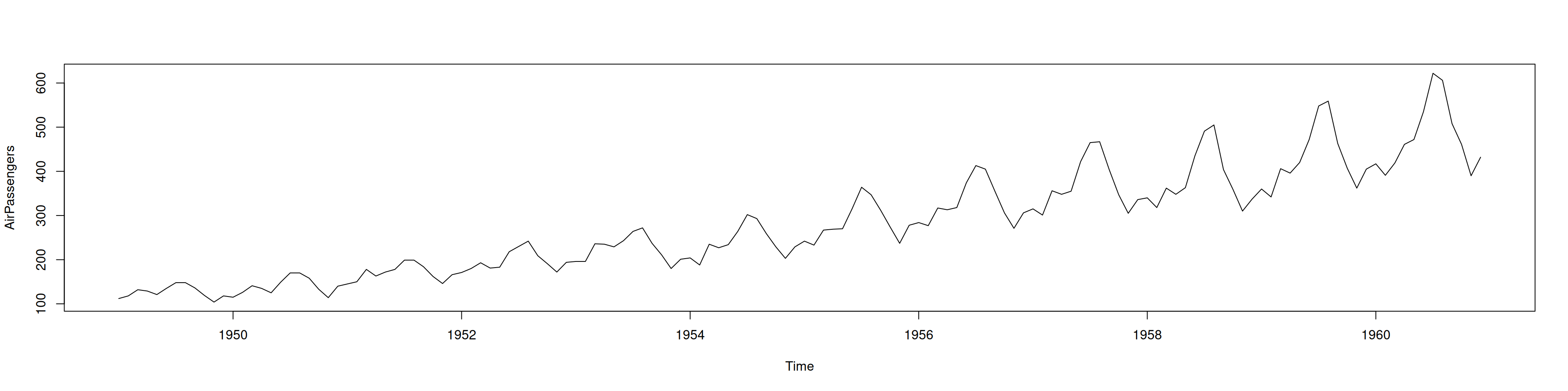

forecast::BoxCox.lambda(AirPassengers, method="guerrero", lower=0)

[1] 4.102259e-05

forecast::BoxCox.lambda(AirPassengers, method="loglik",   lower=0)

[1] 0.2

logAirP = log(AirPassengers)

par(mfrow=c(2,1))
plot(AirPassengers, main="Original")
plot(logAirP,      main="Logaritmo natural")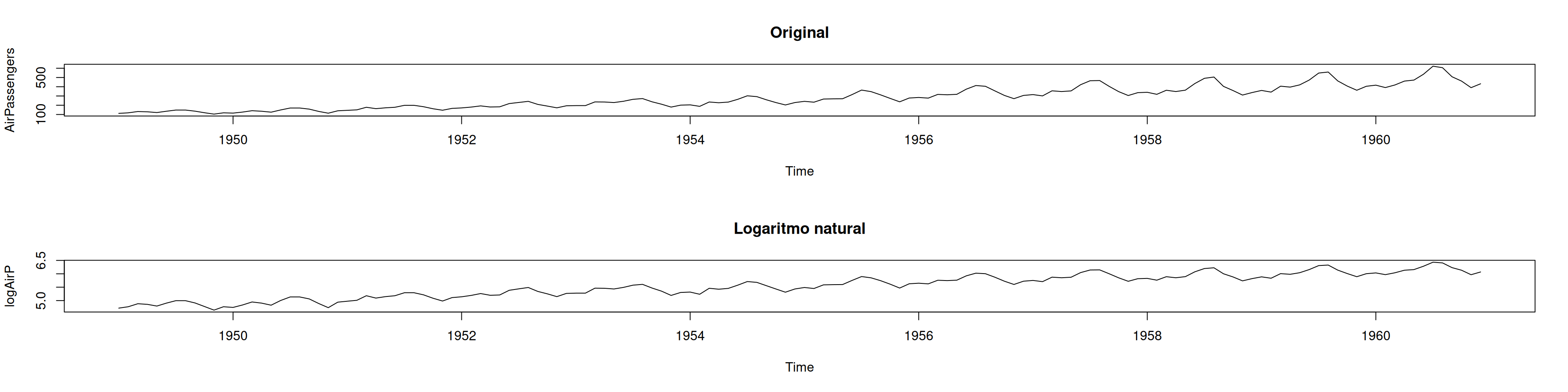

12.3.2 2.2 Detectar raíces unitarias regulares y estacionales

par(mfrow=c(2,1))
acf(logAirP, lag.max = 60)
pacf(logAirP)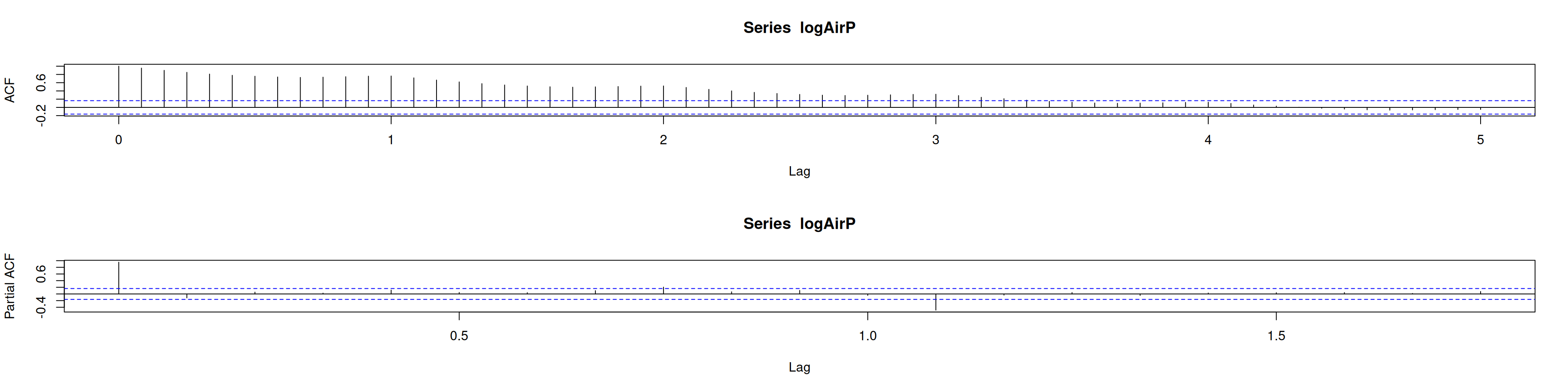

# ADF con drift y tendencia
tseries::adf.test(logAirP)     # p.valor>=0.01 ⇒ no rechaza Ho

Warning in tseries::adf.test(logAirP): p-value smaller than printed p-value

    Augmented Dickey-Fuller Test

data:  logAirP
Dickey-Fuller = -6.4215, Lag order = 5, p-value = 0.01
alternative hypothesis: stationary

# KPSS (Ho: estacionariedad)
tseries::kpss.test(logAirP)    # p.valor<0.05 ⇒ rechaza estacionariedad

Warning in tseries::kpss.test(logAirP): p-value smaller than printed p-value

    KPSS Test for Level Stationarity

data:  logAirP
KPSS Level = 2.8287, Truncation lag parameter = 4, p-value = 0.01

# PP (Ho: raiz unitaria)
tseries::pp.test(logAirP)      # p.valor>=0.01 ⇒ no rechaza Ho

Warning in tseries::pp.test(logAirP): p-value smaller than printed p-value

    Phillips-Perron Unit Root Test

data:  logAirP
Dickey-Fuller Z(alpha) = -47.933, Truncation lag parameter = 4, p-value
= 0.01
alternative hypothesis: stationary

# ADF aumentado
aTSA::adf.test(logAirP, nlag = 8)

Augmented Dickey-Fuller Test 
alternative: stationary 
 
Type 1: no drift no trend 
     lag   ADF p.value
[1,]   0 0.913   0.902
[2,]   1 0.674   0.836
[3,]   2 0.796   0.871
[4,]   3 0.936   0.905
[5,]   4 1.510   0.966
[6,]   5 1.382   0.957
[7,]   6 1.451   0.962
[8,]   7 1.847   0.983
Type 2: with drift no trend 
     lag    ADF p.value
[1,]   0 -1.816   0.400
[2,]   1 -2.018   0.321
[3,]   2 -1.650   0.465
[4,]   3 -1.609   0.481
[5,]   4 -1.288   0.595
[6,]   5 -1.108   0.659
[7,]   6 -0.923   0.723
[8,]   7 -0.807   0.764
Type 3: with drift and trend 
     lag   ADF p.value
[1,]   0 -4.85    0.01
[2,]   1 -7.00    0.01
[3,]   2 -6.71    0.01
[4,]   3 -7.13    0.01
[5,]   4 -5.66    0.01
[6,]   5 -6.42    0.01
[7,]   6 -6.88    0.01
[8,]   7 -6.28    0.01
---- 
Note: in fact, p.value = 0.01 means p.value <= 0.01 

# Decisión de diferencias
ndiffs(logAirP)   # d = 1

[1] 1

nsdiffs(logAirP)  # D = 1

[1] 1

Interpretación:
Se requieren una diferencia regular (\(d=1\)) y una estacional (\(D=1\)) para estacionarizar.

---

12.4 Parte 3: Diferencias y verificación

# Diferencia regular
dlogAirPass = diff(logAirP)

par(mfrow=c(3,1))
plot(AirPassengers); plot(logAirP); plot(dlogAirPass)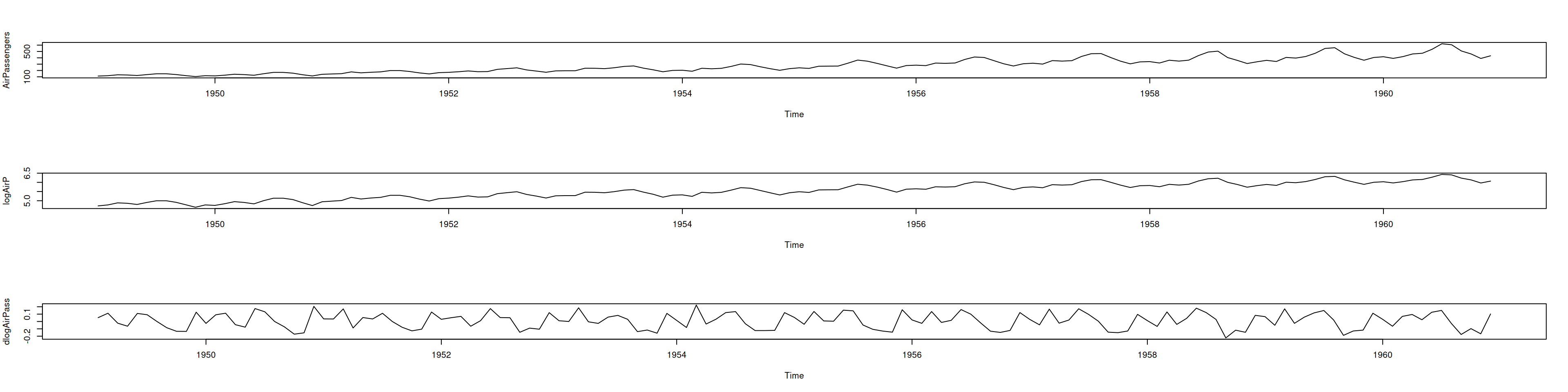

par(mfrow=c(2,1))
acf(dlogAirPass, lag.max = 48)
pacf(dlogAirPass)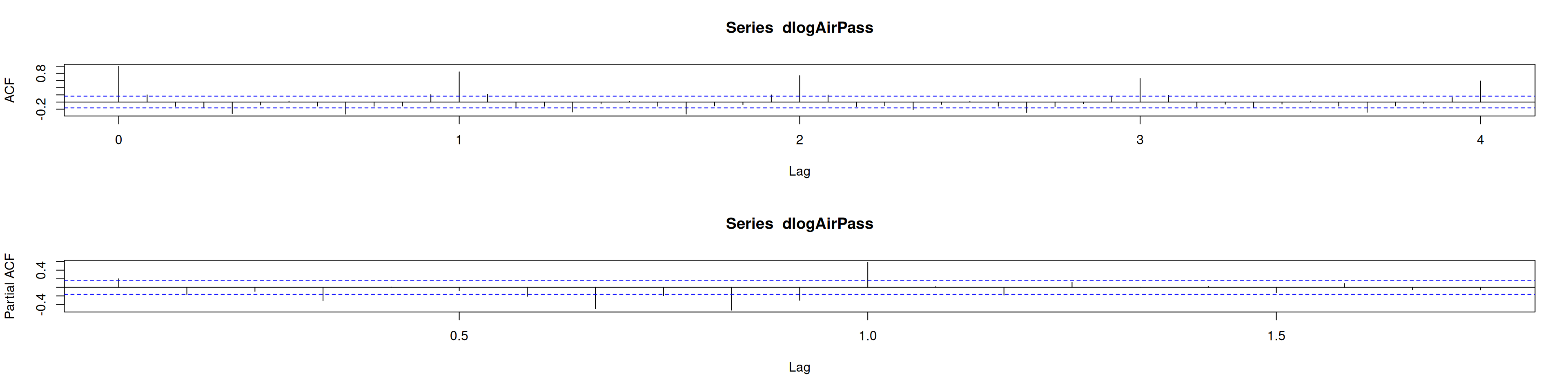

aTSA::adf.test(dlogAirPass, nlag = 15)

Augmented Dickey-Fuller Test 
alternative: stationary 
 
Type 1: no drift no trend 
      lag     ADF p.value
 [1,]   0  -9.606  0.0100
 [2,]   1  -8.816  0.0100
 [3,]   2  -7.634  0.0100
 [4,]   3  -8.745  0.0100
 [5,]   4  -6.791  0.0100
 [6,]   5  -6.245  0.0100
 [7,]   6  -6.571  0.0100
 [8,]   7  -9.498  0.0100
 [9,]   8  -8.028  0.0100
[10,]   9 -10.214  0.0100
[11,]  10  -7.327  0.0100
[12,]  11  -1.868  0.0622
[13,]  12  -1.223  0.2402
[14,]  13  -1.283  0.2186
[15,]  14  -0.992  0.3231
Type 2: with drift no trend 
      lag    ADF p.value
 [1,]   0  -9.63  0.0100
 [2,]   1  -8.86  0.0100
 [3,]   2  -7.71  0.0100
 [4,]   3  -8.94  0.0100
 [5,]   4  -6.98  0.0100
 [6,]   5  -6.46  0.0100
 [7,]   6  -6.91  0.0100
 [8,]   7 -10.55  0.0100
 [9,]   8  -9.57  0.0100
[10,]   9 -15.32  0.0100
[11,]  10 -16.05  0.0100
[12,]  11  -4.60  0.0100
[13,]  12  -3.05  0.0352
[14,]  13  -3.22  0.0222
[15,]  14  -2.72  0.0789
Type 3: with drift and trend 
      lag    ADF p.value
 [1,]   0  -9.60  0.0100
 [2,]   1  -8.83  0.0100
 [3,]   2  -7.69  0.0100
 [4,]   3  -8.92  0.0100
 [5,]   4  -6.95  0.0100
 [6,]   5  -6.43  0.0100
 [7,]   6  -6.88  0.0100
 [8,]   7 -10.51  0.0100
 [9,]   8  -9.55  0.0100
[10,]   9 -15.44  0.0100
[11,]  10 -16.57  0.0100
[12,]  11  -4.94  0.0100
[13,]  12  -3.37  0.0628
[14,]  13  -3.56  0.0392
[15,]  14  -3.12  0.1090
---- 
Note: in fact, p.value = 0.01 means p.value <= 0.01 

# Diferencia estacional
d_dlogAirPass = diff(dlogAirPass, 12)

par(mfrow=c(4,1))
plot(AirPassengers); plot(logAirP); plot(dlogAirPass); plot(d_dlogAirPass)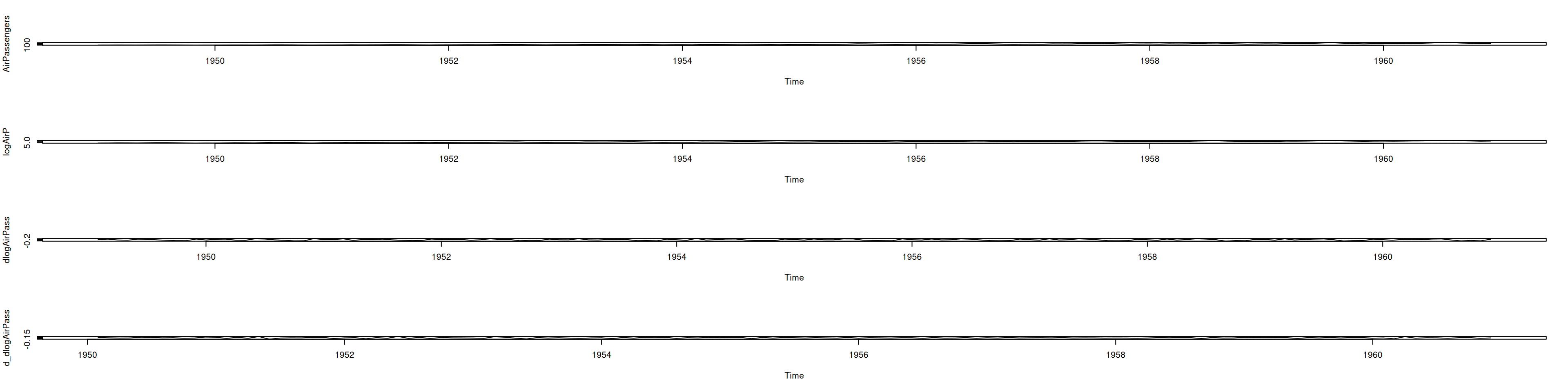

par(mfrow=c(2,1))
acf(d_dlogAirPass, lag.max = 50)
pacf(d_dlogAirPass, lag.max = 50)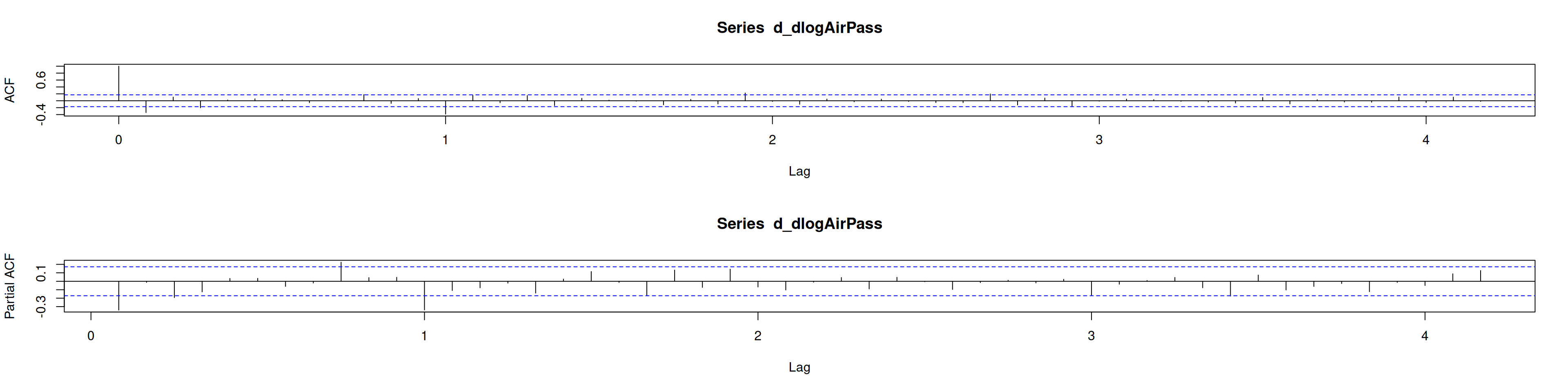

aTSA::adf.test(d_dlogAirPass, nlag = 15)

Augmented Dickey-Fuller Test 
alternative: stationary 
 
Type 1: no drift no trend 
      lag    ADF p.value
 [1,]   0 -16.25    0.01
 [2,]   1  -9.34    0.01
 [3,]   2  -8.65    0.01
 [4,]   3  -7.70    0.01
 [5,]   4  -6.11    0.01
 [6,]   5  -5.23    0.01
 [7,]   6  -5.03    0.01
 [8,]   7  -4.72    0.01
 [9,]   8  -3.38    0.01
[10,]   9  -2.96    0.01
[11,]  10  -2.86    0.01
[12,]  11  -4.39    0.01
[13,]  12  -4.47    0.01
[14,]  13  -4.53    0.01
[15,]  14  -4.03    0.01
Type 2: with drift no trend 
      lag    ADF p.value
 [1,]   0 -16.19  0.0100
 [2,]   1  -9.30  0.0100
 [3,]   2  -8.61  0.0100
 [4,]   3  -7.67  0.0100
 [5,]   4  -6.08  0.0100
 [6,]   5  -5.20  0.0100
 [7,]   6  -5.00  0.0100
 [8,]   7  -4.69  0.0100
 [9,]   8  -3.36  0.0162
[10,]   9  -2.95  0.0452
[11,]  10  -2.84  0.0587
[12,]  11  -4.36  0.0100
[13,]  12  -4.44  0.0100
[14,]  13  -4.51  0.0100
[15,]  14  -4.01  0.0100
Type 3: with drift and trend 
      lag    ADF p.value
 [1,]   0 -16.16  0.0100
 [2,]   1  -9.29  0.0100
 [3,]   2  -8.62  0.0100
 [4,]   3  -7.70  0.0100
 [5,]   4  -6.09  0.0100
 [6,]   5  -5.20  0.0100
 [7,]   6  -5.00  0.0100
 [8,]   7  -4.68  0.0100
 [9,]   8  -3.34  0.0674
[10,]   9  -2.95  0.1816
[11,]  10  -2.82  0.2333
[12,]  11  -4.32  0.0100
[13,]  12  -4.41  0.0100
[14,]  13  -4.48  0.0100
[15,]  14  -3.99  0.0122
---- 
Note: in fact, p.value = 0.01 means p.value <= 0.01 

Interpretación:
Tras \(d=1, D=1\), la serie estacionariza: ACF y PACF ya no muestran picos periódicos ni tendencia.

---

12.5 Parte 4: Ajuste de posibles modelos SARIMA

Se prueban tres modelos con transformación \(\lambda=0\):

# 1) ARIMA(1,1,1)x(0,1,1)[12]
Mod1 = forecast::Arima(
  AirPassengers,
  order    = c(1,1,1),
  seasonal = c(0,1,1),
  lambda   = 0,
  method   = "ML"
)

# 2) ARIMA(0,1,1)x(0,1,1)[12]
Mod2 = forecast::Arima(
  AirPassengers,
  order    = c(0,1,1),
  seasonal = c(0,1,1),
  lambda   = 0,
  method   = "ML"
)

# 3) ARIMA(1,1,0)x(0,1,1)[12]
Mod3 = forecast::Arima(
  AirPassengers,
  order    = c(1,1,0),
  seasonal = c(0,1,1),
  lambda   = 0,
  method   = "ML"
)

Mod2; Mod3

Series: AirPassengers 
ARIMA(0,1,1)(0,1,1)[12] 
Box Cox transformation: lambda= 0 

Coefficients:
          ma1     sma1
      -0.4018  -0.5569
s.e.   0.0896   0.0731

sigma^2 = 0.001371:  log likelihood = 244.7
AIC=-483.4   AICc=-483.21   BIC=-474.77

Series: AirPassengers 
ARIMA(1,1,0)(0,1,1)[12] 
Box Cox transformation: lambda= 0 

Coefficients:
          ar1     sma1
      -0.3395  -0.5619
s.e.   0.0822   0.0748

sigma^2 = 0.001391:  log likelihood = 243.74
AIC=-481.49   AICc=-481.3   BIC=-472.86

Interpretación:
Los criterios AIC/BIC prefieren Mod2: ARIMA(0,1,1)x(0,1,1)[12].

---

12.6 Parte 5: Diagnóstico de Mod2

at_est <- residuals(Mod2)
tsdiag(Mod2)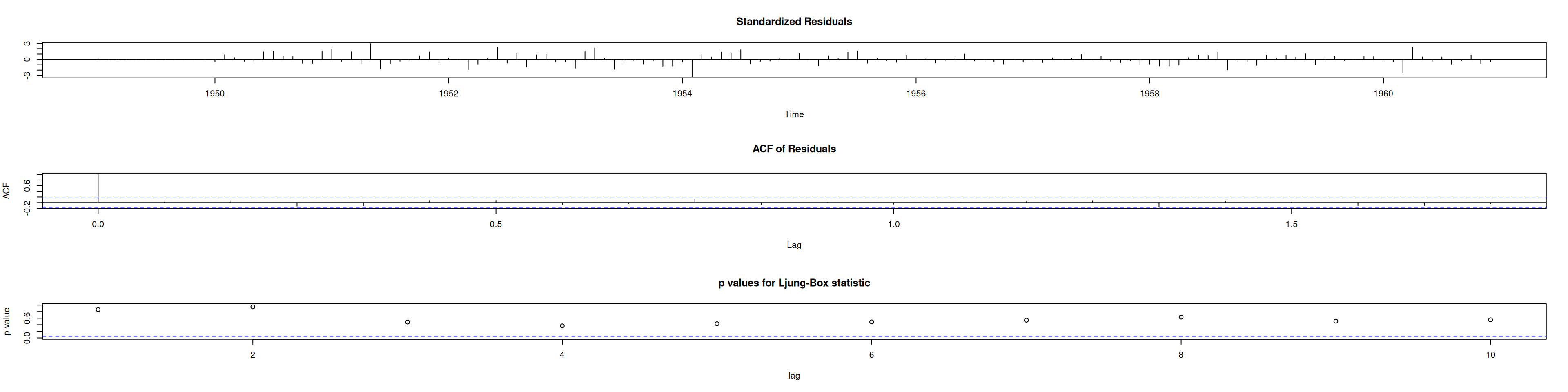

# Normalidad de residuos
library(car); library(nortest)

Loading required package: carData

ad.test(at_est); shapiro.test(at_est)

    Anderson-Darling normality test

data:  at_est
A = 0.68703, p-value = 0.07132

    Shapiro-Wilk normality test

data:  at_est
W = 0.98637, p-value = 0.1674

hist(at_est, freq=FALSE)
lines(density(at_est), col="red", lwd=2)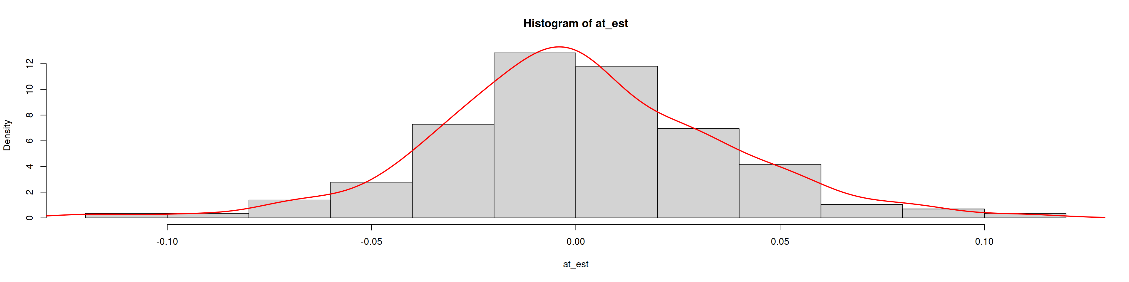

qqnorm(at_est); qqline(at_est, col=2)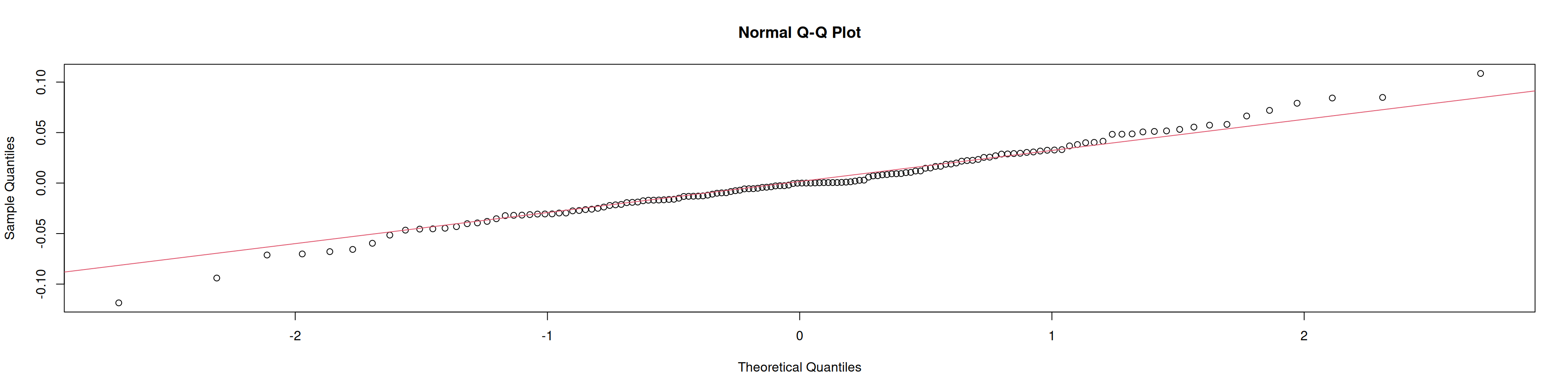

Interpretación:
Residuos no muestran autocorrelación ni alejados de normalidad ⇒ modelo adecuado.

---

12.7 Parte 6: CUSUM y CUSUMQ

cum  = cumsum(at_est)/sd(at_est)
N    = length(at_est)
cumq = cumsum(at_est^2)/sum(at_est^2)
Af   = 0.948  # 95% CUSUM
co   = 0.14013

LS   = Af*sqrt(N) + 2*Af*(1:N)/sqrt(N)
LI   = -LS
LQS  = co + (1:N)/N
LQI  = -co + (1:N)/N

par(mfrow=c(2,1))
plot(cum,  type="l", ylim=c(min(LI),max(LS)), main="CUSUM");  lines(LS, col="red"); lines(LI, col="red")
plot(cumq, type="l", main="CUSUMSQ"); lines(LQS, col="red"); lines(LQI, col="red")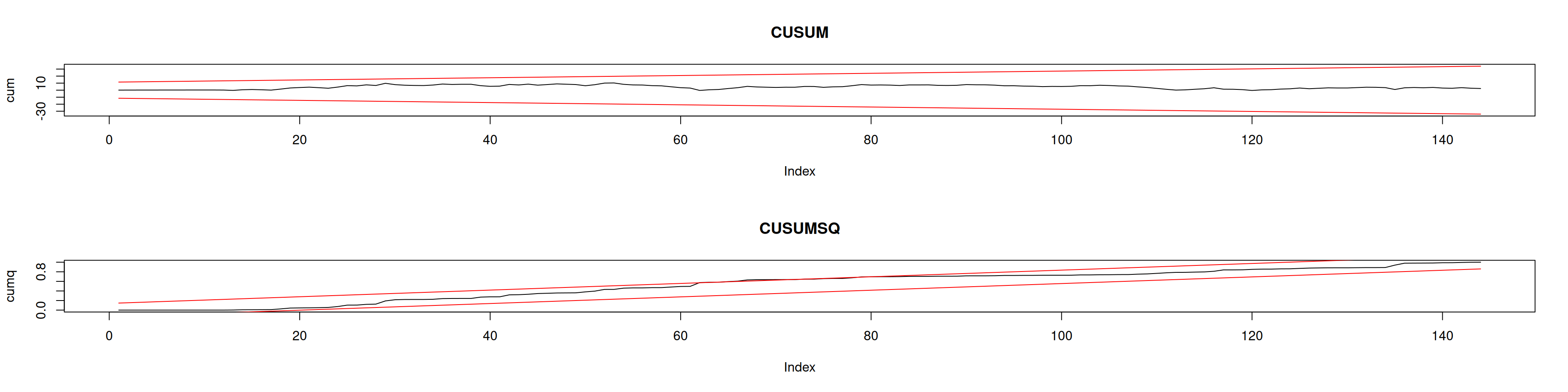

Conclusiones:
- CUSUM: sin cambio estructural.
- CUSUMQ: posible heterocedasticidad moderada ⇒ probar ARCH.

---

12.8 Parte 7: Pronóstico

par(mfrow=c(1,1))
pronosticos12 = forecast::forecast(Mod2, h=12, level=0.95)
plot(pronosticos12)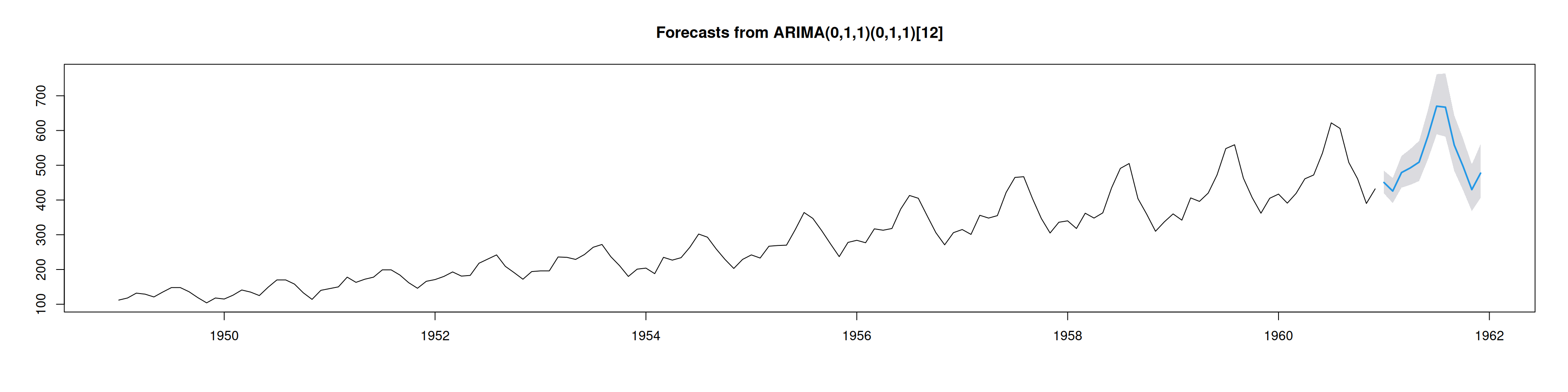

# Con ggplot2
AirPassengers %>%
  forecast::Arima(order=c(0,1,1), seasonal=c(0,1,1), lambda=0, method="ML") %>%
  forecast::forecast(h=12) %>%
  autoplot()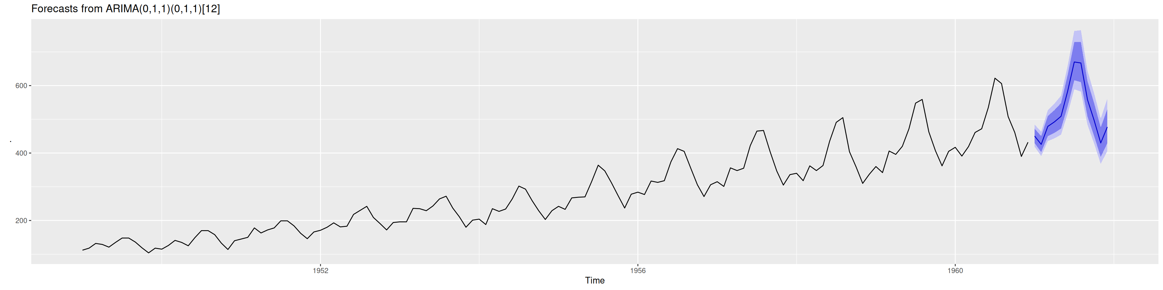

Uso práctico:
Las proyecciones con bandas de confianza guían decisiones de capacidad y planificación en transporte aéreo.

12.8.1 Notas de modelado SARIMA

• Identificar \(d,D\) con ndiffs, nsdiffs.
  
• ACF estacional: picos en múltiplos de 12 ⇒ componente SMA o SAR.
  
• PACF estacional: corte en orden \(P\).
  
• Validar residuos (Ljung–Box, normalidad).
  
• Ajuste iterativo: simplificar términos insignificantes.

Este flujo implementa el método Box–Jenkins para datos estacionales.