Registered S3 method overwritten by 'quantmod':
  method            from
  as.zoo.data.frame zoo
library(TSA)
Registered S3 methods overwritten by 'TSA':
  method       from
  fitted.Arima forecast
  plot.Arima   forecast
Attaching package: 'TSA'
The following objects are masked from 'package:stats':

    acf, arima
The following object is masked from 'package:utils':

    tar
library(readxl)library(tseries)
8.2 Definir directorio y leer datos
# Cambiar "\" por "/" en la ruta#setwd("C:/Users/cubid/Desktop/QUARTO - MATERIAS UNAL/9 SERIES DE TIEMPO/Lesson04")# Leer datos desde Exceldatos <-read_excel("Programa_2_datos.xls", sheet ="Datos")
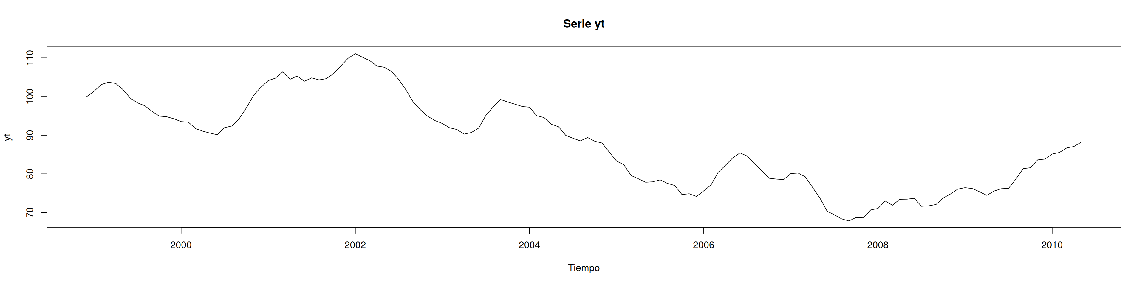
8.3 Preparación de la serie y gráfica inicial
yt <-ts(datos[,2], start =c(1998, 12), frequency =12)plot(yt, type ="l", main ="Serie yt", xlab ="Tiempo")
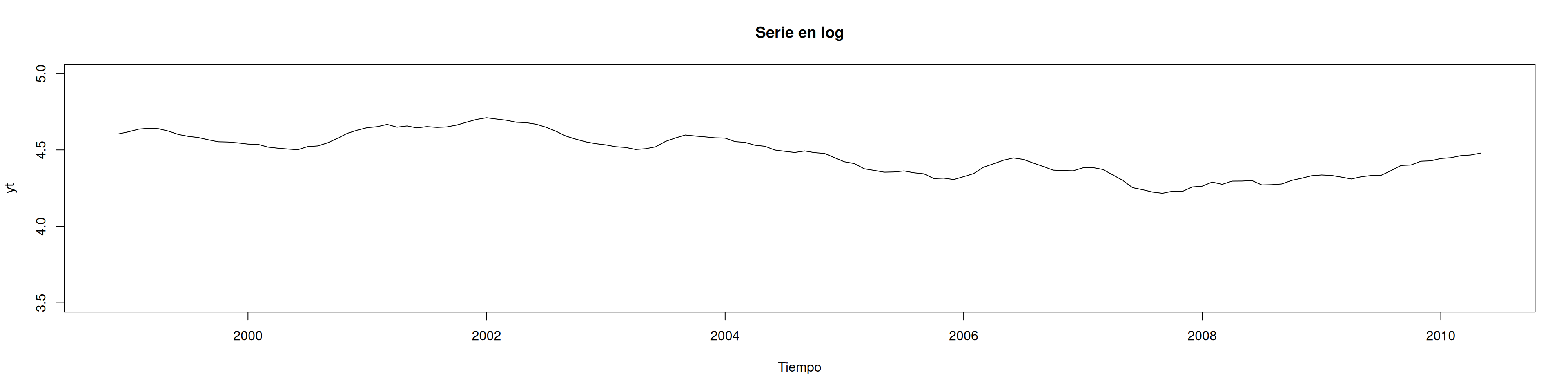
8.4 Transformación logarítmica para estabilizar varianza
ln.yt <-log(yt)plot(ln.yt, type ="l", main ="Serie en log", xlab ="Tiempo", ylim =c(3.5,5))
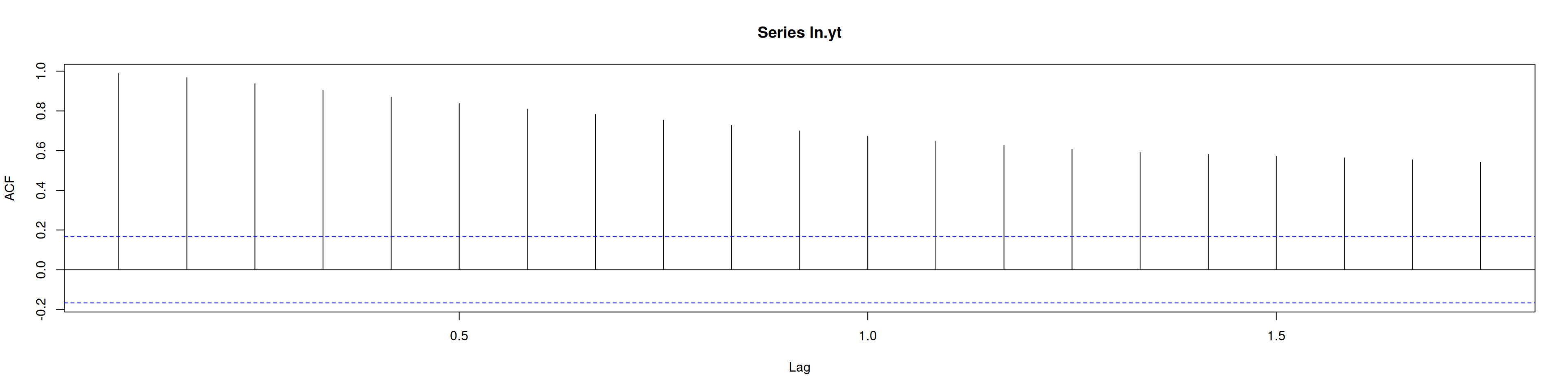
8.5 Prueba de raíz unitaria (ADF)
acf(ln.yt)
adf.test(ln.yt) # Ho: no estacionaria, p-valor>0.05 => no rechaza Ho
    Augmented Dickey-Fuller Test

data:  ln.yt
Dickey-Fuller = -1.4429, Lag order = 5, p-value = 0.8083
alternative hypothesis: stationary
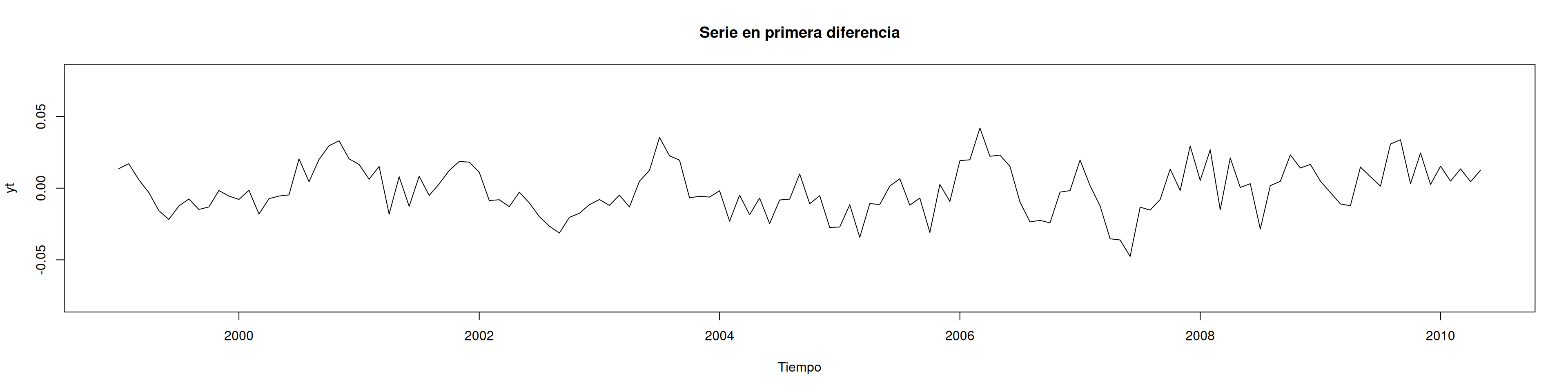
8.6 Primera diferencia para estacionariedad
ytd <-diff(ln.yt, 1)mean(ytd)
[1] -0.000917174
plot(ytd, type ="l", main ="Serie en primera diferencia", xlab ="Tiempo", ylim =c(-0.08,0.08))
adf.test(ytd) # p-valor<0.05 => rechaza Ho
    Augmented Dickey-Fuller Test

data:  ytd
Dickey-Fuller = -3.9839, Lag order = 5, p-value = 0.01215
alternative hypothesis: stationary
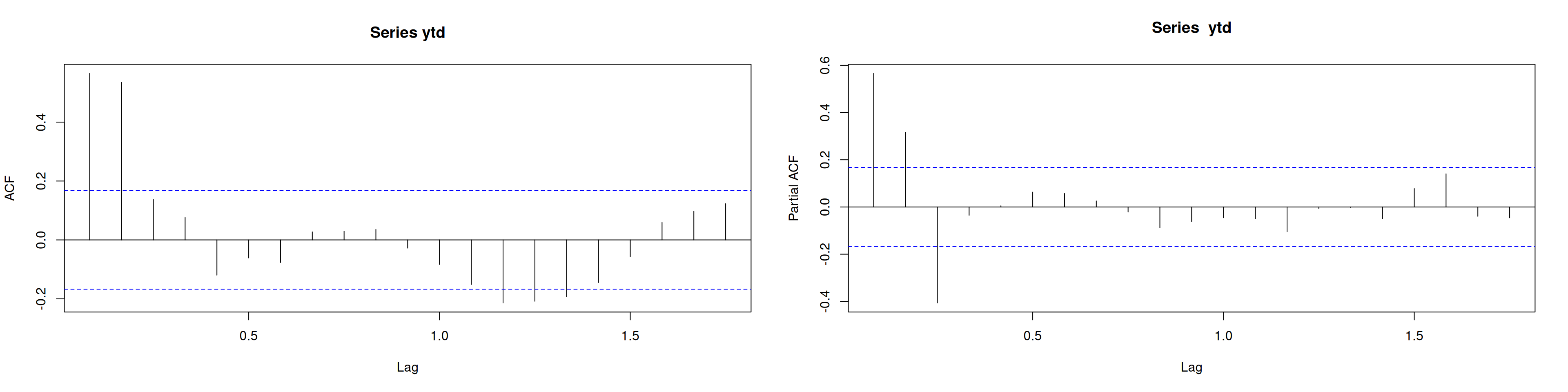
8.7 Identificación: ACF y PACF
par(mfrow =c(1,2))acf(ytd)pacf(ytd)
8.8 Selección de modelo ARMA(p,q)
eacf(ytd) # sugerencia ARMA(3,0)
AR/MA
  0 1 2 3 4 5 6 7 8 9 10 11 12 13
0 x x o o o o o o o o o  o  o  x
1 x x x o x o o o o o o  o  o  o
2 x x o x x o o o o o o  o  o  o
3 o o o o o o o o o o o  o  o  o
4 o o o o o o o o o o o  o  o  o
5 o x o o o o o o o o o  o  o  o
6 x x x o o o o o o o o  o  o  o
7 x x x x o o o o o o o  o  o  o
auto.arima(ytd, trace=TRUE)
 ARIMA(2,0,2)(1,0,1)[12] with non-zero mean : -798.6118
 ARIMA(0,0,0)            with non-zero mean : -723.2355
 ARIMA(1,0,0)(1,0,0)[12] with non-zero mean : -772.0796
 ARIMA(0,0,1)(0,0,1)[12] with non-zero mean : -745.8382
 ARIMA(0,0,0)            with zero mean     : -724.8982
 ARIMA(2,0,2)(0,0,1)[12] with non-zero mean : -800.6425
 ARIMA(2,0,2)            with non-zero mean : -802.8645
 ARIMA(2,0,2)(1,0,0)[12] with non-zero mean : -800.6425
 ARIMA(1,0,2)            with non-zero mean : -801.1236
 ARIMA(2,0,1)            with non-zero mean : -798.6628
 ARIMA(3,0,2)            with non-zero mean : -805.3278
 ARIMA(3,0,2)(1,0,0)[12] with non-zero mean : -803.1612
 ARIMA(3,0,2)(0,0,1)[12] with non-zero mean : -803.1816
 ARIMA(3,0,2)(1,0,1)[12] with non-zero mean : -801.9988
 ARIMA(3,0,1)            with non-zero mean : -807.5113
 ARIMA(3,0,1)(1,0,0)[12] with non-zero mean : -805.3912
 ARIMA(3,0,1)(0,0,1)[12] with non-zero mean : -805.4143
 ARIMA(3,0,1)(1,0,1)[12] with non-zero mean : -804.2908
 ARIMA(3,0,0)            with non-zero mean : -809.47
 ARIMA(3,0,0)(1,0,0)[12] with non-zero mean : -807.3684
 ARIMA(3,0,0)(0,0,1)[12] with non-zero mean : -807.3896
 ARIMA(3,0,0)(1,0,1)[12] with non-zero mean : -806.3672
 ARIMA(2,0,0)            with non-zero mean : -786.8746
 ARIMA(4,0,0)            with non-zero mean : -807.5229
 ARIMA(4,0,1)            with non-zero mean : Inf
 ARIMA(3,0,0)            with zero mean     : -811.5348
 ARIMA(3,0,0)(1,0,0)[12] with zero mean     : -809.4548
 ARIMA(3,0,0)(0,0,1)[12] with zero mean     : -809.4724
 ARIMA(3,0,0)(1,0,1)[12] with zero mean     : -808.3412
 ARIMA(2,0,0)            with zero mean     : -788.9918
 ARIMA(4,0,0)            with zero mean     : -809.607
 ARIMA(3,0,1)            with zero mean     : -809.5951
 ARIMA(2,0,1)            with zero mean     : -800.805
 ARIMA(4,0,1)            with zero mean     : Inf

 Best model: ARIMA(3,0,0)            with zero mean
Series: ytd
ARIMA(3,0,0) with zero mean

Coefficients:
         ar1     ar2      ar3
      0.5166  0.4765  -0.4043
s.e.  0.0772  0.0790   0.0774

sigma^2 = 0.0001495:  log likelihood = 409.92
AIC=-811.84   AICc=-811.53   BIC=-800.16
8.9 Estimación de dos modelos
mod1 <-Arima(ytd, order =c(3,0,0), include.mean =FALSE)summary(mod1)
Series: ytd
ARIMA(3,0,0) with zero mean

Coefficients:
         ar1     ar2      ar3
      0.5166  0.4765  -0.4043
s.e.  0.0772  0.0790   0.0774

sigma^2 = 0.0001495:  log likelihood = 409.92
AIC=-811.84   AICc=-811.53   BIC=-800.16

Training set error measures:
                        ME       RMSE         MAE      MPE     MAPE      MASE
Training set -0.0003684491 0.01209189 0.009562996 39.69704 126.5415 0.4781506
                    ACF1
Training set -0.01678247
mod2 <-Arima(ytd, order =c(2,0,1), include.mean =FALSE)summary(mod2)
Series: ytd
ARIMA(2,0,1) with zero mean

Coefficients:
          ar1     ar2     ma1
      -0.0941  0.6311  0.5533
s.e.   0.1002  0.0704  0.1114

sigma^2 = 0.000162:  log likelihood = 404.55
AIC=-801.11   AICc=-800.81   BIC=-789.43

Training set error measures:
                        ME       RMSE        MAE      MPE     MAPE      MASE
Training set -0.0002526163 0.01258662 0.01008932 37.02357 119.4948 0.5044668
                   ACF1
Training set 0.08053776
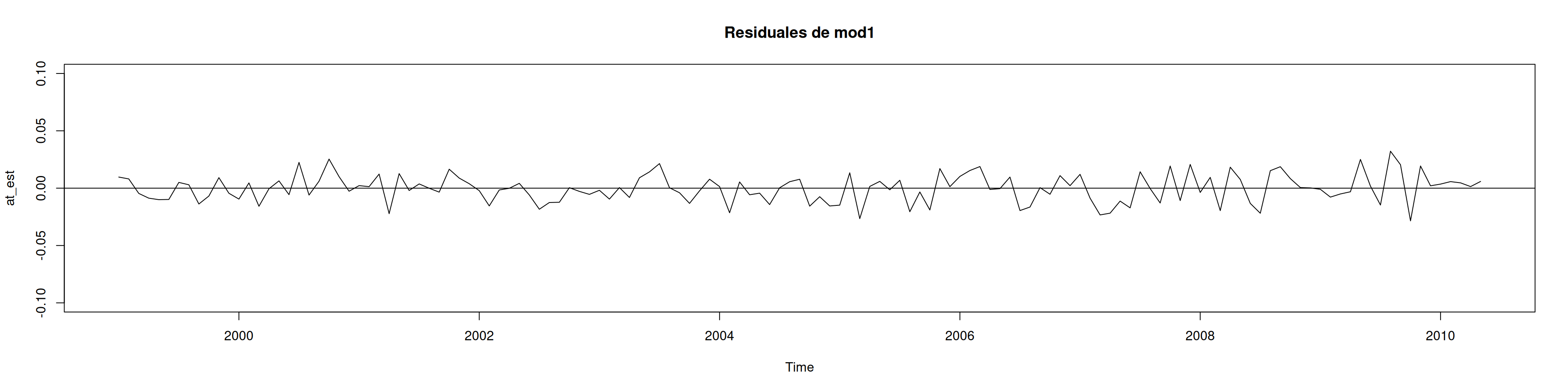
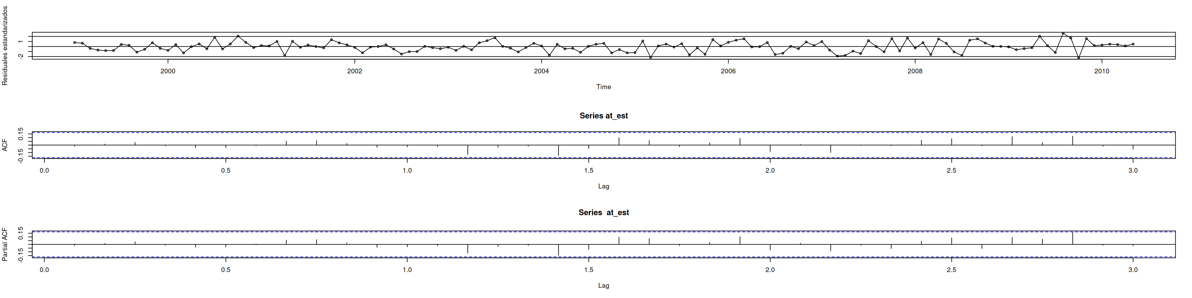
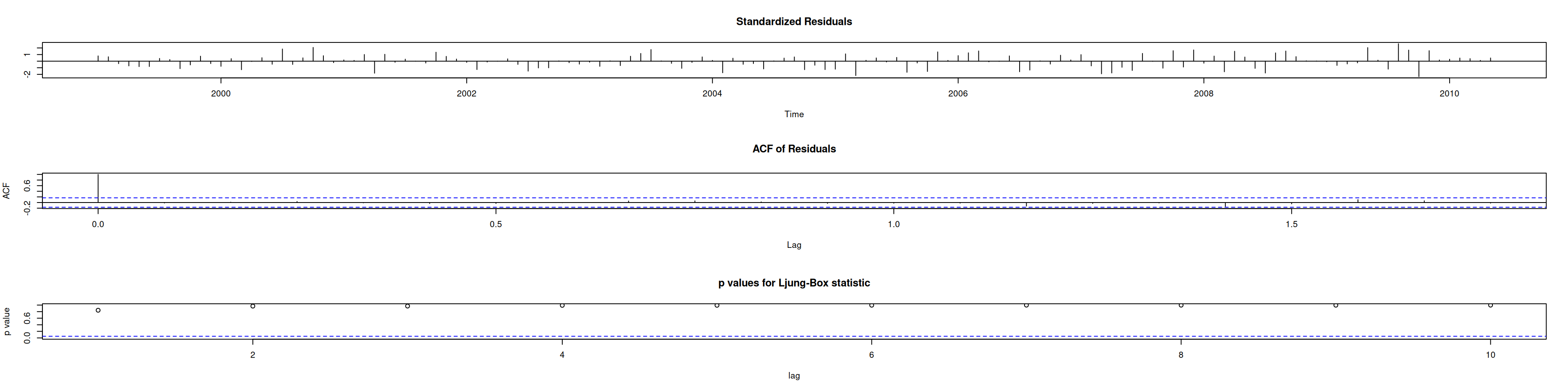
8.10 Diagnóstico del modelo 1
at_est <-residuals(mod1)# Residuales y residuales estandarizadosplot(at_est, ylim =c(-0.1,0.1), main ="Residuales de mod1"); abline(h=0)
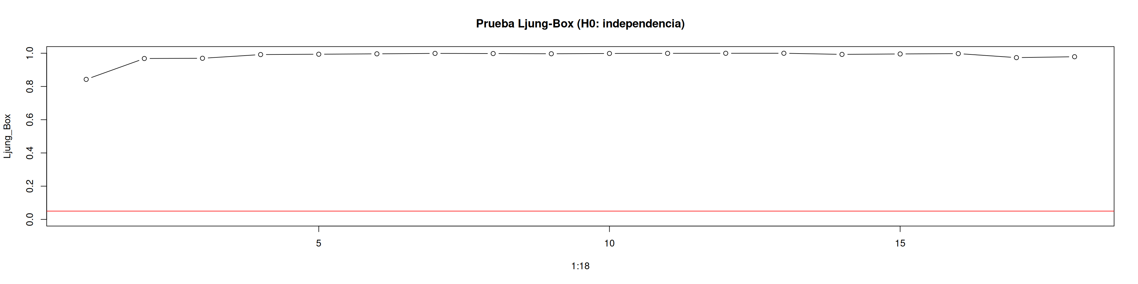
# Para varios rezagosLjung_Box <-sapply(1:18, function(i) Box.test(at_est, lag = i, type ="Ljung")$p.value)colnames(Ljung_Box) <-NULLdata.frame(Rezago =1:18, p.valor =round(Ljung_Box, 4))
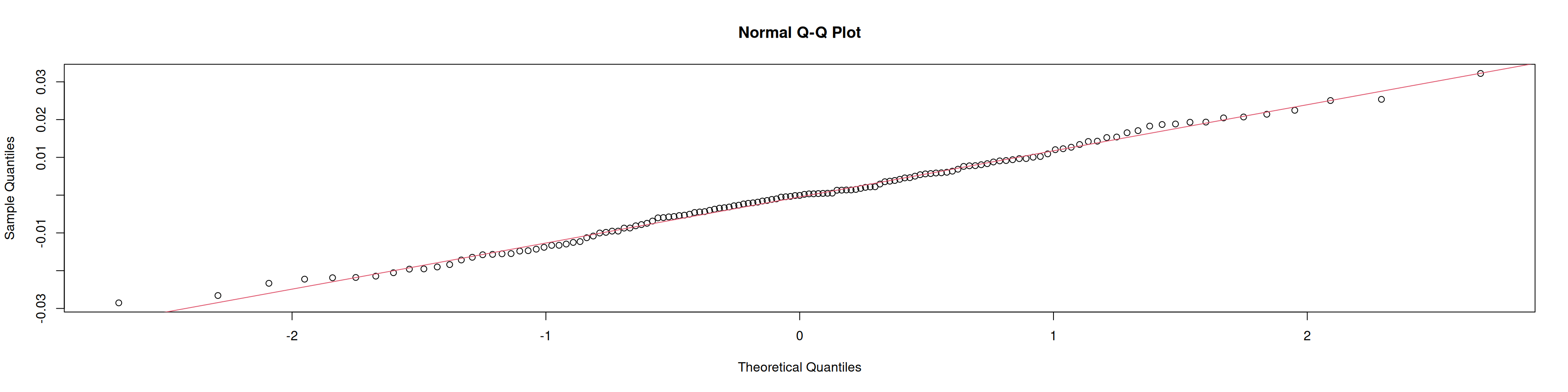
library(nortest)ad.test(at_est) # p-valor>0.05: no rechaza normalidad
    Anderson-Darling normality test

data:  at_est
A = 0.22546, p-value = 0.8166
shapiro.test(at_est) # idem
    Shapiro-Wilk normality test

data:  at_est
W = 0.99377, p-value = 0.8164
qqnorm(at_est); qqline(at_est, col =2)
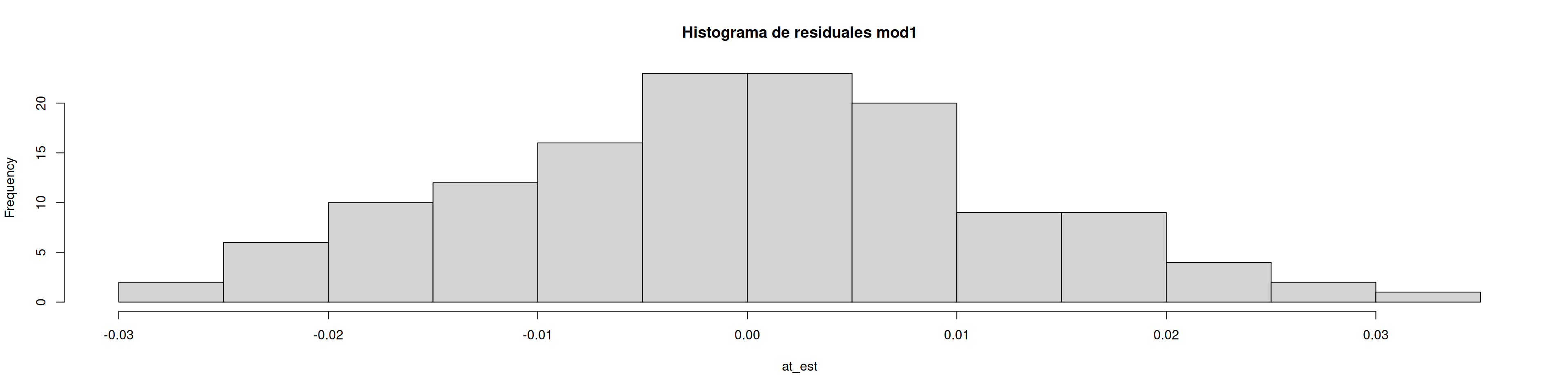
hist(at_est, main ="Histograma de residuales mod1")
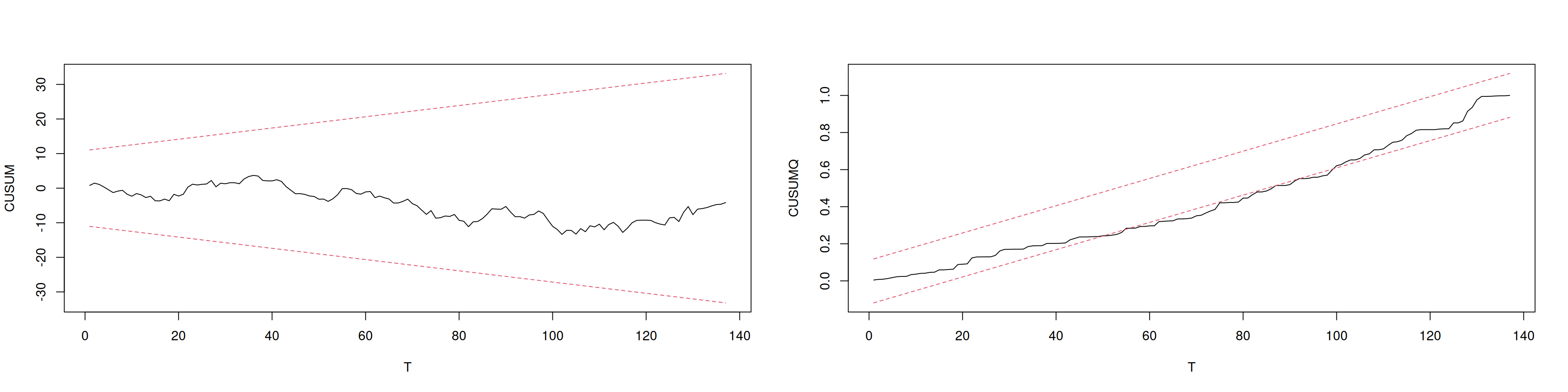
8.13 Función CUSUM y CUSUMQ
cucuq <-function(x, nivel) { A <-0.948 N <-length(x) T <-1:N cu <-cumsum(x) /sd(x) LS <- A *sqrt(N-1) +2*A*(T-1)/sqrt(N-1) LI <--LS cu2 <-cumsum(x^2) /sum(x^2) LS2 <- nivel + (T-1)/(N-1) LI2 <--nivel + (T-1)/(N-1)par(mfrow =c(1,2))matplot(T, cbind(cu, LS, LI), type="l", lty=c(1,2,2),ylab="CUSUM", col=c(1,2,2))matplot(T, cbind(cu2, LS2, LI2), type="l", lty=c(1,2,2),ylab="CUSUMQ", col=c(1,2,2))}cucuq(at_est, nivel =0.11848)
8.14 Evaluación predictiva dentro y fuera de muestra
# Dentro de muestrasummary(mod1)
Series: ytd
ARIMA(3,0,0) with zero mean

Coefficients:
         ar1     ar2      ar3
      0.5166  0.4765  -0.4043
s.e.  0.0772  0.0790   0.0774

sigma^2 = 0.0001495:  log likelihood = 409.92
AIC=-811.84   AICc=-811.53   BIC=-800.16

Training set error measures:
                        ME       RMSE         MAE      MPE     MAPE      MASE
Training set -0.0003684491 0.01209189 0.009562996 39.69704 126.5415 0.4781506
                    ACF1
Training set -0.01678247
summary(mod2)
Series: ytd
ARIMA(2,0,1) with zero mean

Coefficients:
          ar1     ar2     ma1
      -0.0941  0.6311  0.5533
s.e.   0.1002  0.0704  0.1114

sigma^2 = 0.000162:  log likelihood = 404.55
AIC=-801.11   AICc=-800.81   BIC=-789.43

Training set error measures:
                        ME       RMSE        MAE      MPE     MAPE      MASE
Training set -0.0002526163 0.01258662 0.01008932 37.02357 119.4948 0.5044668
                   ACF1
Training set 0.08053776
# Fuera de muestradatos.evalua <-read_excel("Programa_2_datos.xls", sheet ="Evaluar")yt.eval <-ts(datos.evalua[,2], start =c(2010, 12), frequency =12)mod1.evalua <-Arima(yt.eval, model = mod1)mod2.evalua <-Arima(yt.eval, model = mod2)accuracy(mod1.evalua)
                   ME     RMSE      MAE      MPE     MAPE MASE        ACF1
Training set 39.11233 39.99697 39.11233 42.00275 42.00275  NaN -0.04246928
accuracy(mod2.evalua)
                   ME     RMSE      MAE      MPE     MAPE MASE      ACF1
Training set 31.63266 33.46823 31.63266 34.05565 34.05565  NaN 0.1746239
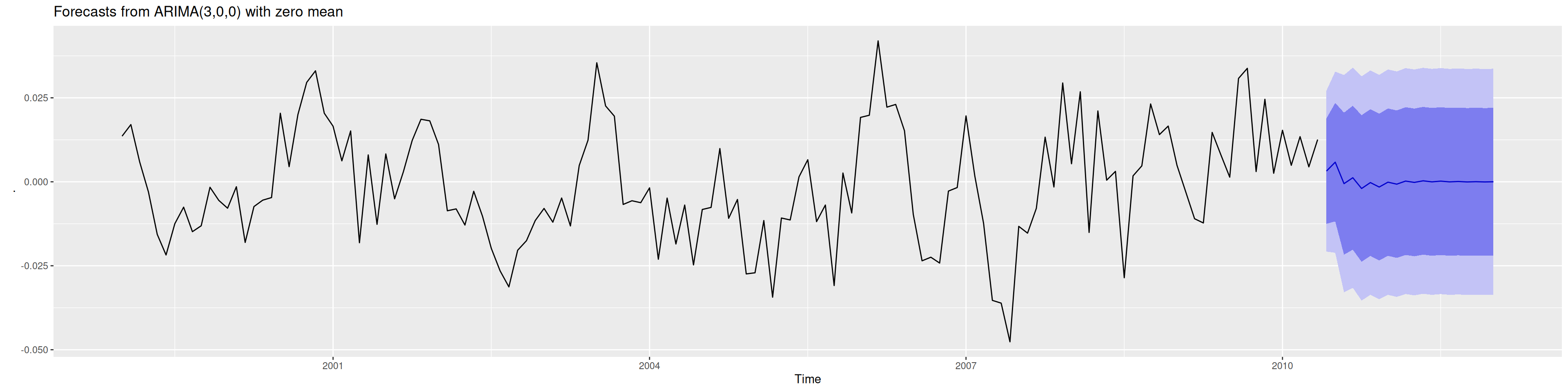
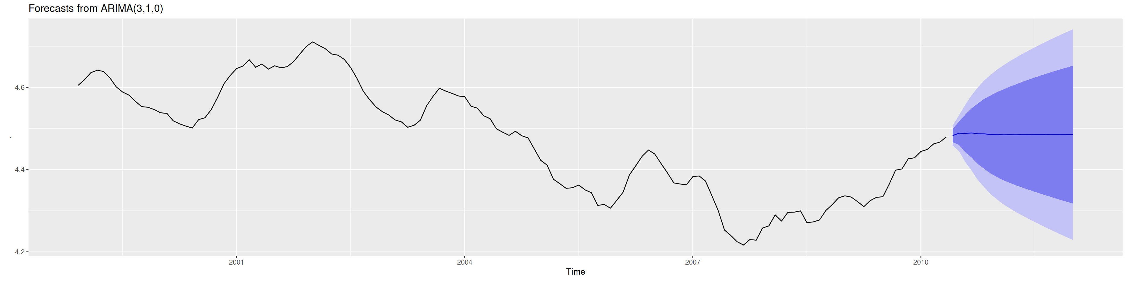
---title: "ARMA - Box-Jenkins"author: "Brayan Cubides"toc: truetoc-location: righttoc-depth: 2#number-sections: truecode-tools: truelightbox: trueself-contained: false ---## Limpieza de entorno y carga de librerías```{r, fig.width=20, fig.height=5, out.width="100%"}rm(list =ls(all =TRUE))library(forecast)library(TSA)library(readxl)library(tseries)```## Definir directorio y leer datos```{r, fig.width=20, fig.height=5, out.width="100%"}# Cambiar "\" por "/" en la ruta#setwd("C:/Users/cubid/Desktop/QUARTO - MATERIAS UNAL/9 SERIES DE TIEMPO/Lesson04")# Leer datos desde Exceldatos <-read_excel("Programa_2_datos.xls", sheet ="Datos")```## Preparación de la serie y gráfica inicial```{r, fig.width=20, fig.height=5, out.width="100%"}yt <-ts(datos[,2], start =c(1998, 12), frequency =12)plot(yt, type ="l", main ="Serie yt", xlab ="Tiempo")```## Transformación logarítmica para estabilizar varianza```{r, fig.width=20, fig.height=5, out.width="100%"}ln.yt <-log(yt)plot(ln.yt, type ="l", main ="Serie en log", xlab ="Tiempo", ylim =c(3.5,5))```## Prueba de raíz unitaria (ADF)```{r, fig.width=20, fig.height=5, out.width="100%"}acf(ln.yt)adf.test(ln.yt) # Ho: no estacionaria, p-valor>0.05 => no rechaza Ho```## Primera diferencia para estacionariedad```{r, fig.width=20, fig.height=5, out.width="100%"}ytd <-diff(ln.yt, 1)mean(ytd)plot(ytd, type ="l", main ="Serie en primera diferencia", xlab ="Tiempo", ylim =c(-0.08,0.08))adf.test(ytd) # p-valor<0.05 => rechaza Ho```## Identificación: ACF y PACF```{r, fig.width=20, fig.height=5, out.width="100%"}par(mfrow =c(1,2))acf(ytd)pacf(ytd)```## Selección de modelo ARMA(p,q)```{r, fig.width=20, fig.height=5, out.width="100%"}eacf(ytd) # sugerencia ARMA(3,0)auto.arima(ytd, trace=TRUE)```## Estimación de dos modelos```{r, fig.width=20, fig.height=5, out.width="100%"}mod1 <-Arima(ytd, order =c(3,0,0), include.mean =FALSE)summary(mod1)mod2 <-Arima(ytd, order =c(2,0,1), include.mean =FALSE)summary(mod2)```## Diagnóstico del modelo 1```{r, fig.width=20, fig.height=5, out.width="100%"}at_est <-residuals(mod1)# Residuales y residuales estandarizadosplot(at_est, ylim =c(-0.1,0.1), main ="Residuales de mod1"); abline(h=0)par(mfrow =c(3,1))plot(rstandard(mod1), type ="o", ylab ="Residuales estandarizados"); abline(h =c(-2,0,2))acf(at_est, lag.max =36)pacf(at_est, lag.max =36)```## Prueba de Ljung-Box```{r, fig.width=20, fig.height=5, out.width="100%"}# Para varios rezagosLjung_Box <-sapply(1:18, function(i) Box.test(at_est, lag = i, type ="Ljung")$p.value)colnames(Ljung_Box) <-NULLdata.frame(Rezago =1:18, p.valor =round(Ljung_Box, 4))plot(1:18, Ljung_Box, type="b", main="Prueba Ljung-Box (H0: independencia)", ylim=c(0,1))abline(h =0.05, col ="red")``````{r, fig.width=20, fig.height=5, out.width="100%"}# tsdiag hace diagnóstico completotsdiag(mod1)```## Normalidad de residuales```{r, fig.width=20, fig.height=5, out.width="100%"}library(nortest)ad.test(at_est) # p-valor>0.05: no rechaza normalidadshapiro.test(at_est) # idemqqnorm(at_est); qqline(at_est, col =2)hist(at_est, main ="Histograma de residuales mod1")```## Función CUSUM y CUSUMQ```{r, fig.width=20, fig.height=5, out.width="100%"}cucuq <-function(x, nivel) { A <-0.948 N <-length(x) T <-1:N cu <-cumsum(x) /sd(x) LS <- A *sqrt(N-1) +2*A*(T-1)/sqrt(N-1) LI <--LS cu2 <-cumsum(x^2) /sum(x^2) LS2 <- nivel + (T-1)/(N-1) LI2 <--nivel + (T-1)/(N-1)par(mfrow =c(1,2))matplot(T, cbind(cu, LS, LI), type="l", lty=c(1,2,2),ylab="CUSUM", col=c(1,2,2))matplot(T, cbind(cu2, LS2, LI2), type="l", lty=c(1,2,2),ylab="CUSUMQ", col=c(1,2,2))}cucuq(at_est, nivel =0.11848)```## Evaluación predictiva dentro y fuera de muestra```{r, fig.width=20, fig.height=5, out.width="100%"}# Dentro de muestrasummary(mod1)summary(mod2)# Fuera de muestradatos.evalua <-read_excel("Programa_2_datos.xls", sheet ="Evaluar")yt.eval <-ts(datos.evalua[,2], start =c(2010, 12), frequency =12)mod1.evalua <-Arima(yt.eval, model = mod1)mod2.evalua <-Arima(yt.eval, model = mod2)accuracy(mod1.evalua)accuracy(mod2.evalua)```## Pronósticos con ggplot2```{r, fig.width=20, fig.height=5, out.width="100%"}library(ggplot2)library(forecast)# Pronóstico de diferenciasytd %>%Arima(order =c(3,0,0), include.mean =FALSE) %>%forecast(h =20) %>%autoplot()# Pronóstico en nivelesln.yt %>%Arima(order =c(3,1,0), include.mean =FALSE) %>%forecast(h =20) %>%autoplot()```